This is the abstract class for generating instances of axes with various types of plots from one or more columns of data.
More...
This is the abstract class for generating instances of axes with various types of plots from one or more columns of data.
While it can be directly used for visualization tasks, this class primarily serves as the superclass for the visualization subclasses accessible to the end users.
- Note
- In case of pm.vis.SubplotContour, pm.vis.SubplotContour3, and pm.vis.SubplotContourf visualization objects, the density of the input data is first computed and smoothed by a Gaussian kernel density estimator and then passed to the MATLAB intrinsic plotting functions
contour, contourf, contour3.
Dynamic class attributes
This class contains a set of attributes that are defined dynamically at runtime for the output object depending on its subclass (plot type it represents).
The following is the list of all class attributes that are dynamically added to the instantiated class objects based on the specified input plot type.
See also the explicit class and superclass attributes not listed below.
-
colx (standing for x-columns; available for all axes types)
Optional property that determines the columns of the specified dataframe to serve as the x-values. It can have multiple forms:
-
a numeric or cell array of column indices in the input
dfref.
-
a string or cell array of column names in
dfref.Properties.VariableNames.
-
a cell array of a mix of the above two.
-
a numeric range.
If colx is empty,
-
it will be set to the row indices of
dfref for line/scatter axes types.
-
it will be set to all columns of
dfref for density axes types.
- Warning
- In all cases,
colx must have a length that is either 0 (empty), 1, or equal to the length of coly or colz.
If the length is 1, then colx will be plotted against data corresponding to each element of coly and colz.
Example usage ⛓
Subplot.colx = [
"sampleLogFunc",
"sampleVariable1"]
Subplot.colx = {
"sampleLogFunc", 9,
"sampleVariable1"}
Subplot.colx = 7:9 # every column in the data frame starting from column #7 to #9
Subplot.colx = 7:2:20 # every other column in the data frame starting from column #7 to #20
This is the abstract class for generating instances of axes with various types of plots from one or m...
-
coly (standing for y-columns; available for all axes types except pm.vis.SubplotHeatmap, pm.vis.SubplotHistogram, pm.vis.SubplotHistfit)
Optional property that determines the columns of the specified dataframe to serve as the z-values.
It can have multiple forms:
-
a numeric or cell array of column indices in the input
dfref.
-
a string or cell array of column names in
dfref.Properties.VariableNames.
-
a cell array of a mix of the above two.
-
a numeric range.
If coly is empty,
-
it will be set to the row indices of
dfref for line/scatter axes types.
-
it will be set to all columns of
dfref for density axes types.
- Warning
- In all cases,
coly must have a length that is either 0 (empty), 1, or equal to the length of colx or colz.
If the length is 1, then coly will be plotted against data corresponding to each element of colx and colz.
Example usage ⛓
Subplot.coly = [
"sampleLogFunc",
"sampleVariable1"]
Subplot.coly = {
"sampleLogFunc", 9,
"sampleVariable1"}
Subplot.coly = 7:9 # every column in the data frame starting from column #7 to #9
Subplot.coly = 7:2:20 # every other column in the data frame starting from column #7 to #20
-
colz (standing for z-columns; available only for 3D plots, e.g., pm.vis.SubplotLine3, pm.vis.SubplotScatter3, pm.vis.SubplotLineScatter3)
Optional property that determines the columns of the specified dataframe to serve as the z-values.
It can have multiple forms:
-
a numeric or cell array of column indices in the input
dfref.
-
a string or cell array of column names in
dfref.Properties.VariableNames.
-
a cell array of a mix of the above two.
-
a numeric range.
If colz is empty,
-
it will be set to the row indices of
dfref for line/scatter axes types.
-
it will be set to all columns of
dfref for density axes types.
- Warning
- In all cases,
colz must have a length that is either 0 (empty), 1, or equal to the length of colx or coly.
If the length is 1, then colz will be plotted against data corresponding to each element of colx and coly.
Example usage ⛓
Subplot.colz = [
"sampleLogFunc",
"sampleVariable1"]
Subplot.colz = {
"sampleLogFunc", 9,
"sampleVariable1"}
Subplot.colz = 7:9 % every column in the data frame starting from column #7 to #9
Subplot.colz = 7:2:20 % every other column in the data frame starting from column #7 to #20
-
colc (standing for color-columns; available only for 2D/3D line/scatter axes types, e.g., pm.vis.SubplotLine3, pm.vis.SubplotScatter3, pm.vis.SubplotLineScatter3, pm.vis.SubplotLine, pm.vis.SubplotScatter, pm.vis.SubplotLineScatter)
Optional property that determines the columns of the input dfref to use as the color mapping values for each line/point element in the plot.
It can have multiple forms:
-
a numeric or cell array of column indices in the input
dfref.
-
a string or cell array of column names in
dfref.Properties.VariableNames.
-
a cell array of a mix of the above two.
-
a numeric range.
The default value is the indices of the rows of the input dfref.
Example usage ⛓
Subplot.colc = [
"sampleLogFunc",
"sampleVariable1"]
Subplot.colc = {
"sampleLogFunc", 9,
"sampleVariable1"}
Subplot.colc = 7:9 # every column in the data frame starting from column #7 to #9
Subplot.colc = 7:2:20 # every other column in the data frame starting from column #7 to #20
- Note
- For example usage, see the documentation of the constructor of the class pm.vis.Subplot::Subplot.
- Developer Remark:
- While dynamic addition of class attributes is not ideal, the current design was deemed unavoidable and best, given the constraints of the MATLAB language and visualization tools.
- See also
- pm.vis
pm.vis.axes.Axes
pm.matlab.Handle
pm.vis.Cascade
pm.vis.Subplot
pm.vis.Triplex
pm.vis.Figure
pm.vis.Plot
pm.vis.Tile
Final Remarks ⛓
If you believe this algorithm or its documentation can be improved, we appreciate your contribution and help to edit this page's documentation and source file on GitHub.
For details on the naming abbreviations, see this page.
For details on the naming conventions, see this page.
This software is distributed under the MIT license with additional terms outlined below.
-
If you use any parts or concepts from this library to any extent, please acknowledge the usage by citing the relevant publications of the ParaMonte library.
-
If you regenerate any parts/ideas from this library in a programming environment other than those currently supported by this ParaMonte library (i.e., other than C, C++, Fortran, MATLAB, Python, R), please also ask the end users to cite this original ParaMonte library.
This software is available to the public under a highly permissive license.
Help us justify its continued development and maintenance by acknowledging its benefit to society, distributing it, and contributing to it.
- Copyright
- Computational Data Science Lab
- Author:
- Fatemeh Bagheri, May 20 2024, 1:25 PM, NASA Goddard Space Flight Center (GSFC), Washington, D.C.
Amir Shahmoradi, May 16 2016, 9:03 AM, Oden Institute for Computational Engineering and Sciences (ICES), UT Austin
Definition at line 187 of file Subplot.m.
| function Subplot::Subplot |
( |
in |
ptype, |
|
|
in |
dfref, |
|
|
in |
varargin |
|
) |
| |
Construct and return an object of class pm.vis.Subplot.
This is the custom constructor of the class pm.vis.Subplot.
- Parameters
-
| [in] | ptype | : See the documentation of the corresponding input argument of the superclass constructor pm.vis.axes.Axes::Axes.
|
| [in] | dfref | : The input MATLAB matrix or table containing the data to plot or a function handle that returns such a MATLAB matrix or table.
Specifying a function handle is superior to specifying the data directly, because the function handle will always use the most updated version of the user table or matrix.
(optional. The default is an empty table.) |
| [in] | varargin | : Any property, value pair of the parent object.
If the property is a struct(), then its value must be given as a cell array, with consecutive elements representing the struct property-name, property-value pairs.
Note that all of these property-value pairs can be also directly set via the parent object attributes, before calling the make() method.
The input varargin can also contain the components of the subplot component of the parent object.
|
- Returns
self : The output scalar object of class pm.vis.Subplot.
Possible calling interfaces ⛓
s = pm.vis.Subplot(ptype,
dfref);
s = pm.vis.Subplot(ptype,
dfref, varargin);
- Warning
- In all cases,
colc must have a length that is either 0, or 1, or equal to the maximum lengths of (colx, coly, colz).
If the length is 1, then all data will be plotted with the same color mapping determined by values specified by the elements of colc.
If it is an empty object having length 0, then the default value will be used.
- Note
- In case of pm.vis.SubplotContour/pm.vis.SubplotContourf/pm.vis.SubplotContour3 visualization objects, the density of the input data is first computed and smoothed by a Gaussian kernel density estimator and then passed to the MATLAB intrinsic plotting functions ,
contour, contourf, contour3.
Example usage ⛓
1cd(fileparts(mfilename(
'fullpath'))); % Change working directory to source code directory.
2addpath(
'../../../'); % Add the ParaMonte library
root directory to the search path.
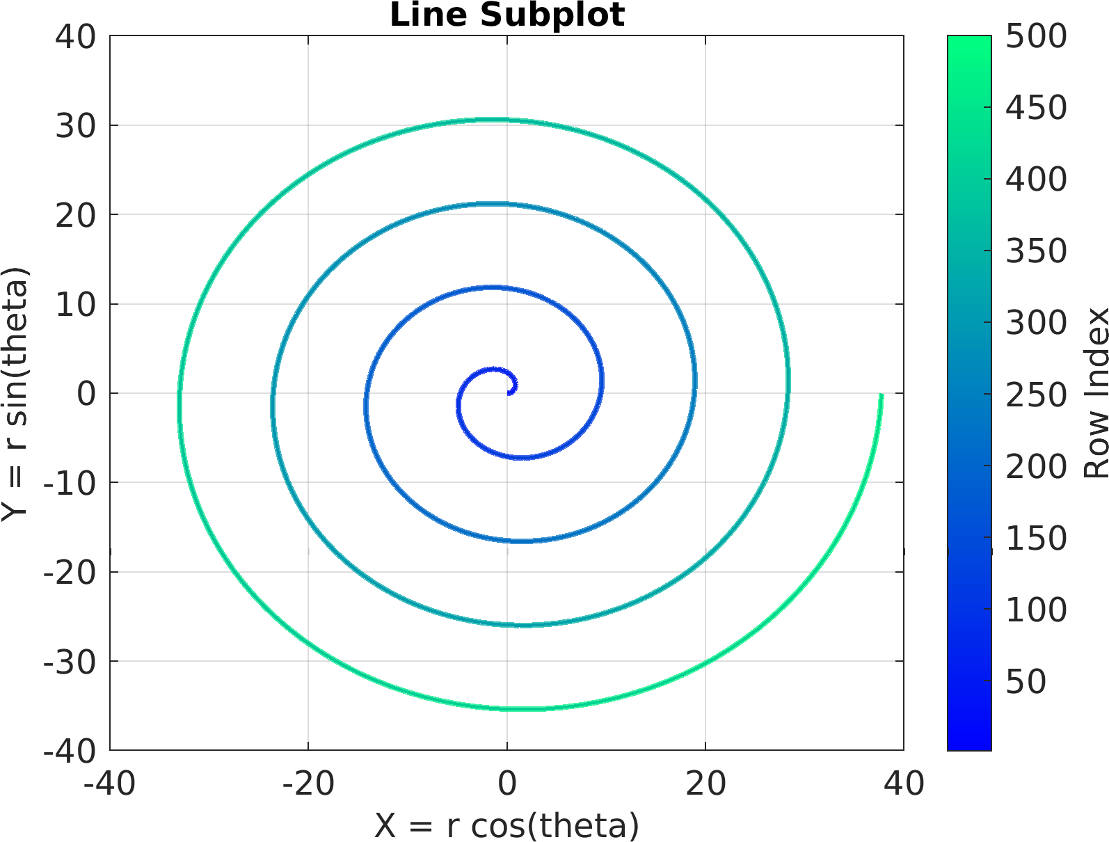
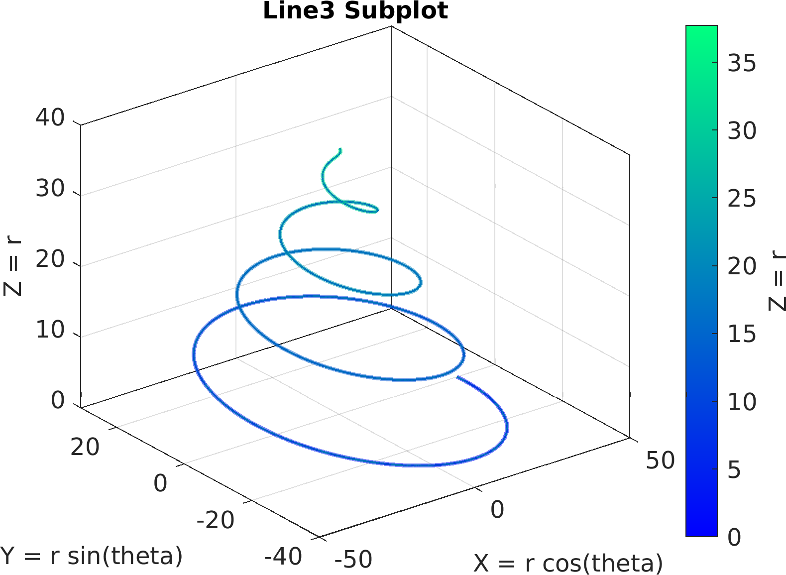
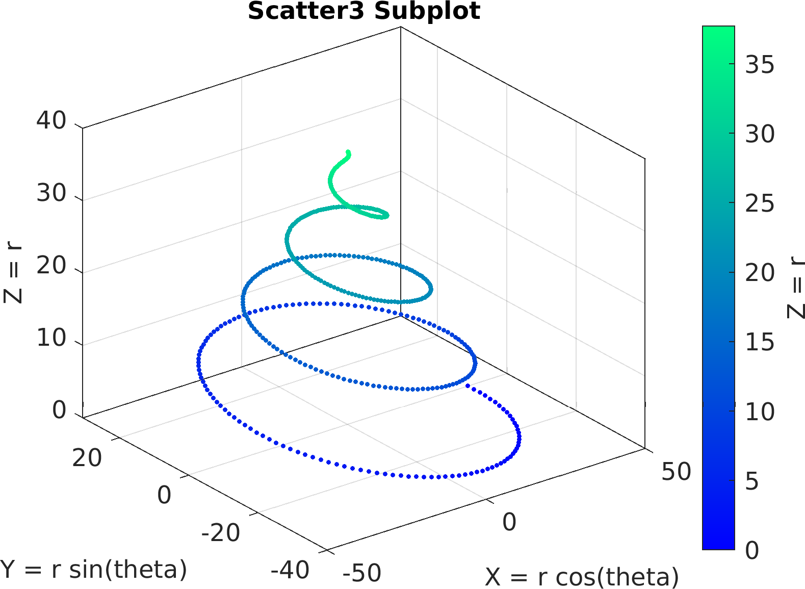
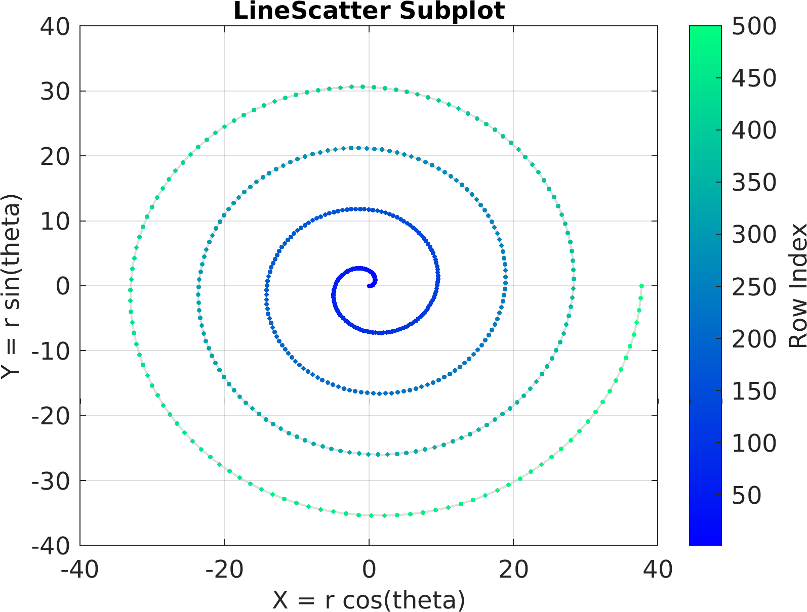
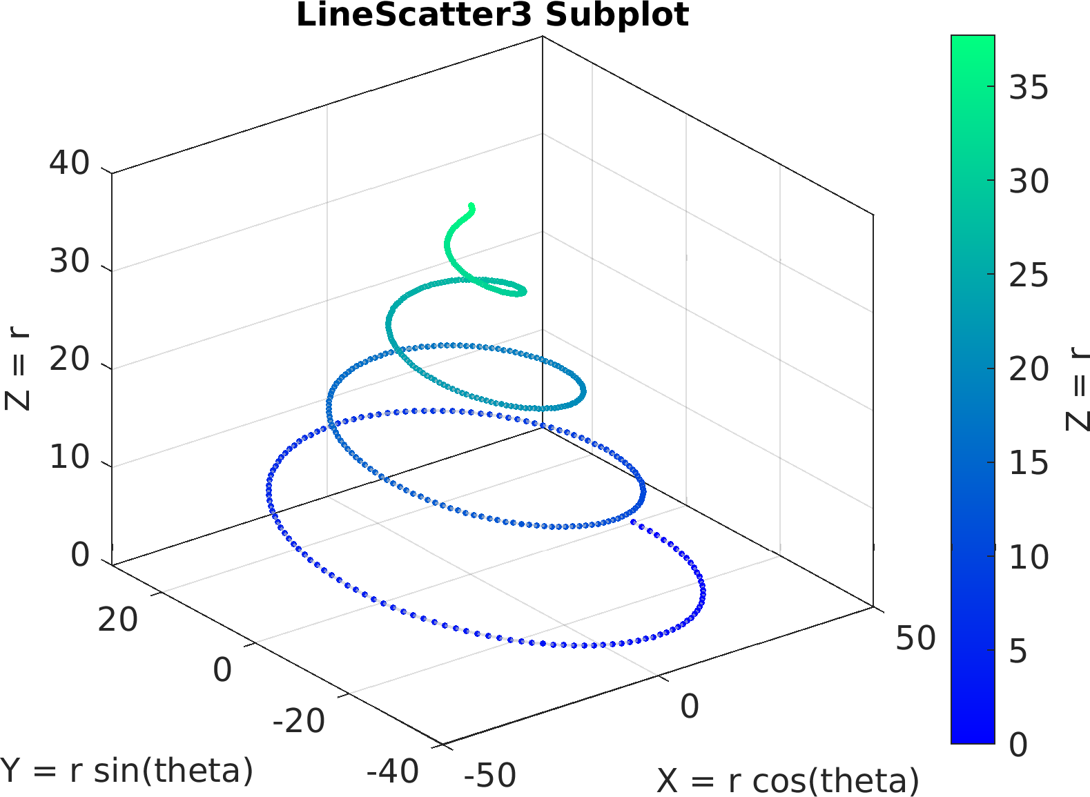
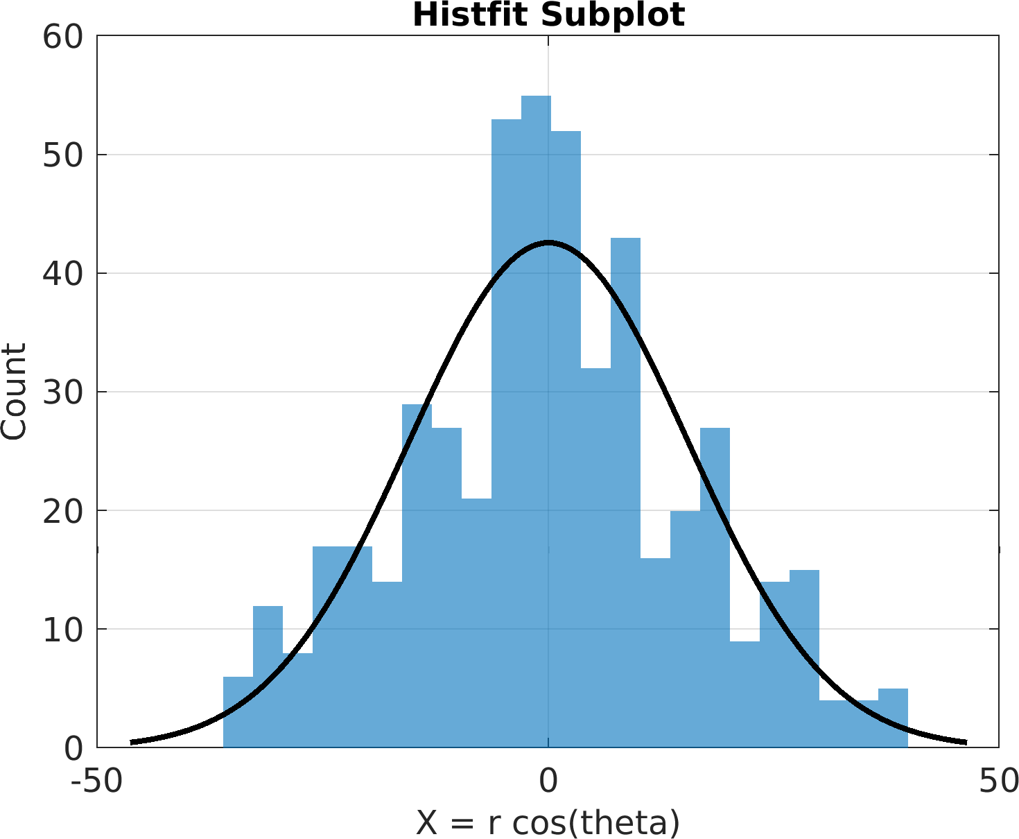
4theta = linspace(0, 8 * pi, 500);
6df = array2table(ctranspose([r .* cos(theta); r .* sin(theta); r(end) - r]));
7df.Properties.VariableNames = [
"X = r cos(theta)",
"Y = r sin(theta)",
"Z = r"];
9figure(
"color",
"white");
10sv = pm.vis.Subplot(
"Line", df);
11sv.title.titletext =
"Line Subplot";
12sv.surface.lineWidth = 2;
13sv.make(
"colx", 1,
"coly", 2);
14pm.vis.figure.savefig(
"SubplotLine.1.png",
"-m3");
16figure(
"color",
"white");
17sv = pm.vis.Subplot(
"Line3", df);
18sv.title.titletext =
"Line3 Subplot";
19sv.surface.lineWidth = 2;
20sv.make(
"colx", 1,
"coly", 2,
"colz", 3);
21pm.vis.figure.savefig(
"SubplotLine3.1.png",
"-m3");
23figure(
"color",
"white");
24sv = pm.vis.Subplot(
"Scatter", df);
25sv.title.titletext =
"Scatter Subplot";
26sv.make(
"colx", 1,
"coly", 2);
27pm.vis.figure.savefig(
"SubplotScatter.1.png",
"-m3");
29figure(
"color",
"white");
30sv = pm.vis.Subplot(
"Scatter3", df);
31sv.title.titletext =
"Scatter3 Subplot";
32sv.make(
"colx", 1,
"coly", 2,
"colz", 3);
33pm.vis.figure.savefig(
"SubplotScatter3.1.png",
"-m3");
35figure(
"color",
"white");
36sv = pm.vis.Subplot(
"LineScatter", df);
37sv.title.titletext =
"LineScatter Subplot";
38sv.make(
"colx", 1,
"coly", 2);
39pm.vis.figure.savefig(
"SubplotLineScatter.1.png",
"-m3");
41figure(
"color",
"white");
42sv = pm.vis.Subplot(
"LineScatter3", df);
43sv.title.titletext =
"LineScatter3 Subplot";
44sv.make(
"colx", 1,
"coly", 2,
"colz", 3);
45pm.vis.figure.savefig(
"SubplotLineScatter3.1.png",
"-m3");
47figure(
"color",
"white");
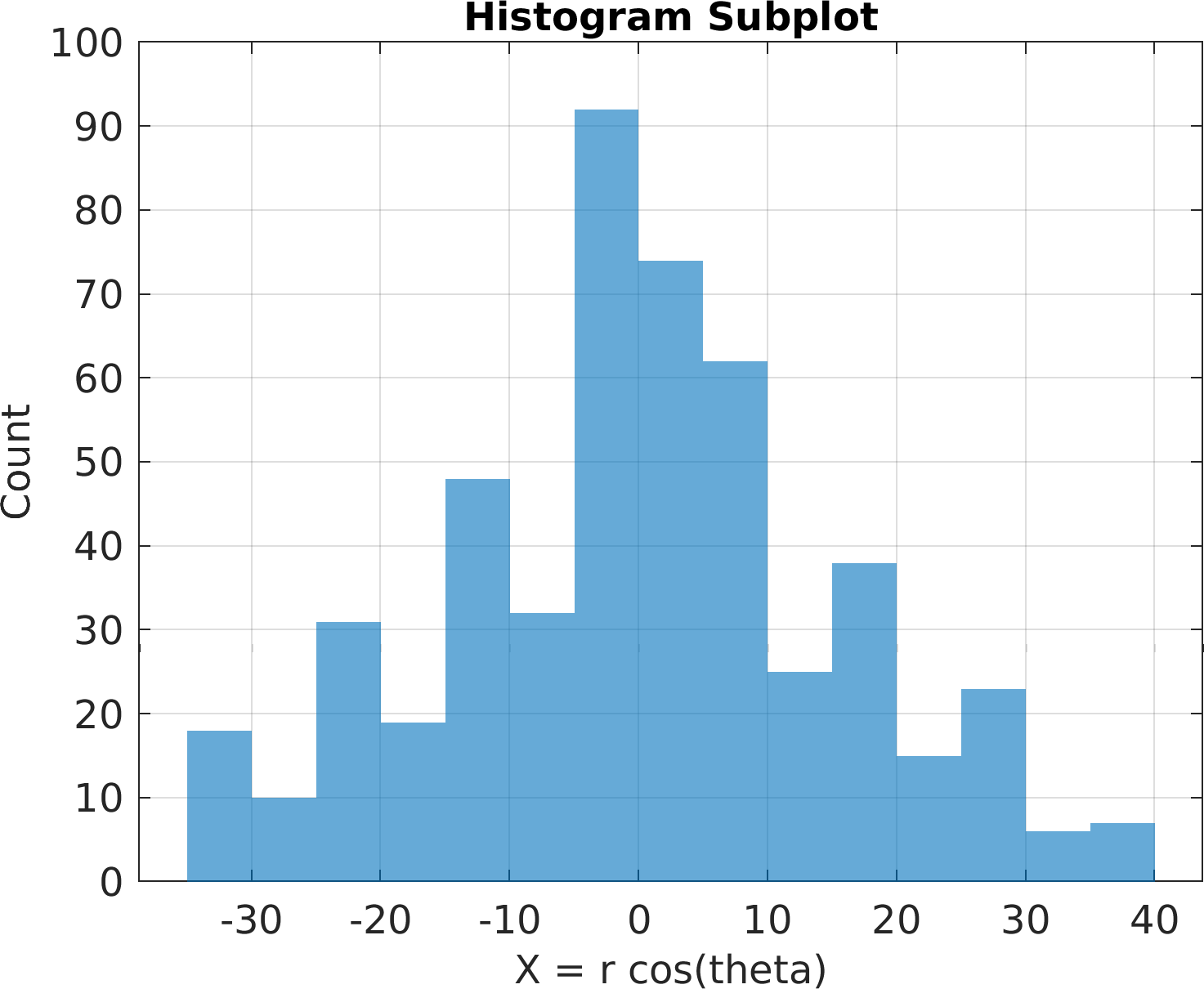
48sv = pm.vis.Subplot(
"Histogram", df);
49sv.title.titletext =
"Histogram Subplot";
51pm.vis.figure.savefig(
"SubplotHistogram.1.png",
"-m3");
53figure(
"color",
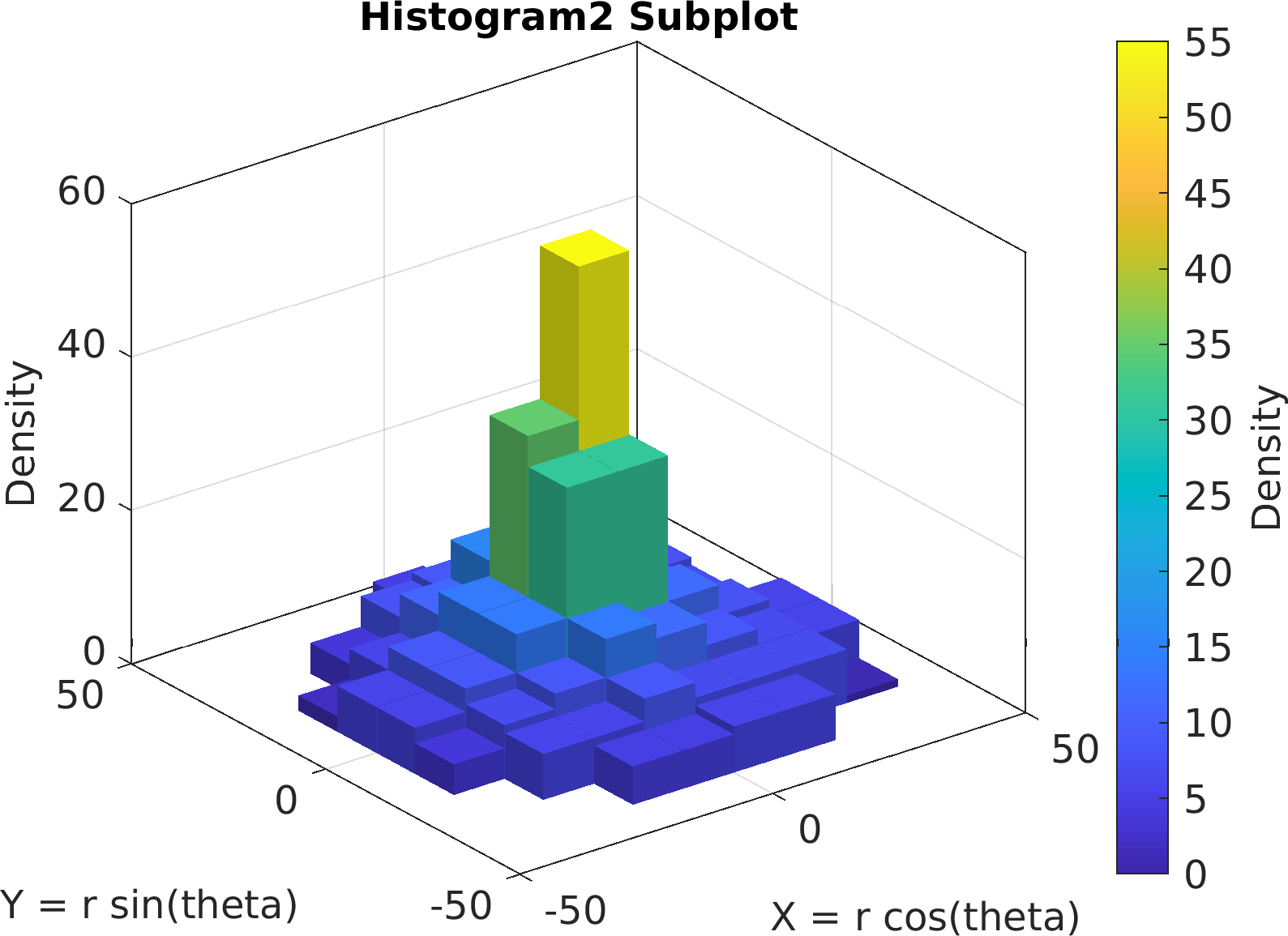
"white");
54sv = pm.vis.Subplot(
"Histogram2", df);
55sv.title.titletext =
"Histogram2 Subplot";
56sv.make(
"colx", 1,
"coly", 2);
57pm.vis.figure.savefig(
"SubplotHistogram2.1.png",
"-m3");
59figure(
"color",
"white");
60sv = pm.vis.Subplot(
"Histfit", df);
61sv.title.titletext =
"Histfit Subplot";
63pm.vis.figure.savefig(
"SubplotHistfit.1.png",
"-m3");
65figure(
"color",
"white");
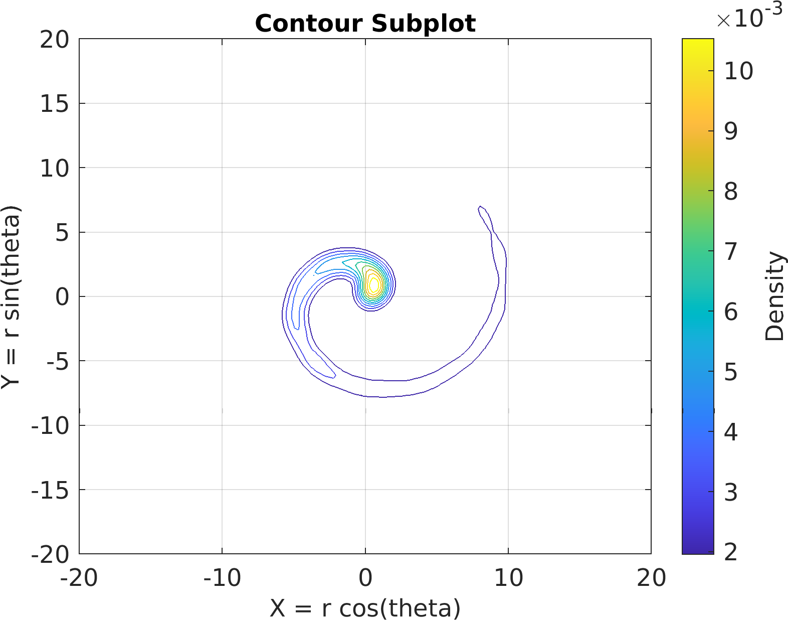
66sv = pm.vis.Subplot(
"Contour", df);
67sv.title.titletext =
"Contour Subplot";
68sv.make(
"colx", 1,
"coly", 2,
"xlim", [-20, 20],
"ylim", [-20, 20]);
69pm.vis.figure.savefig(
"SubplotContour.1.png",
"-m3");
71figure(
"color",
"white");
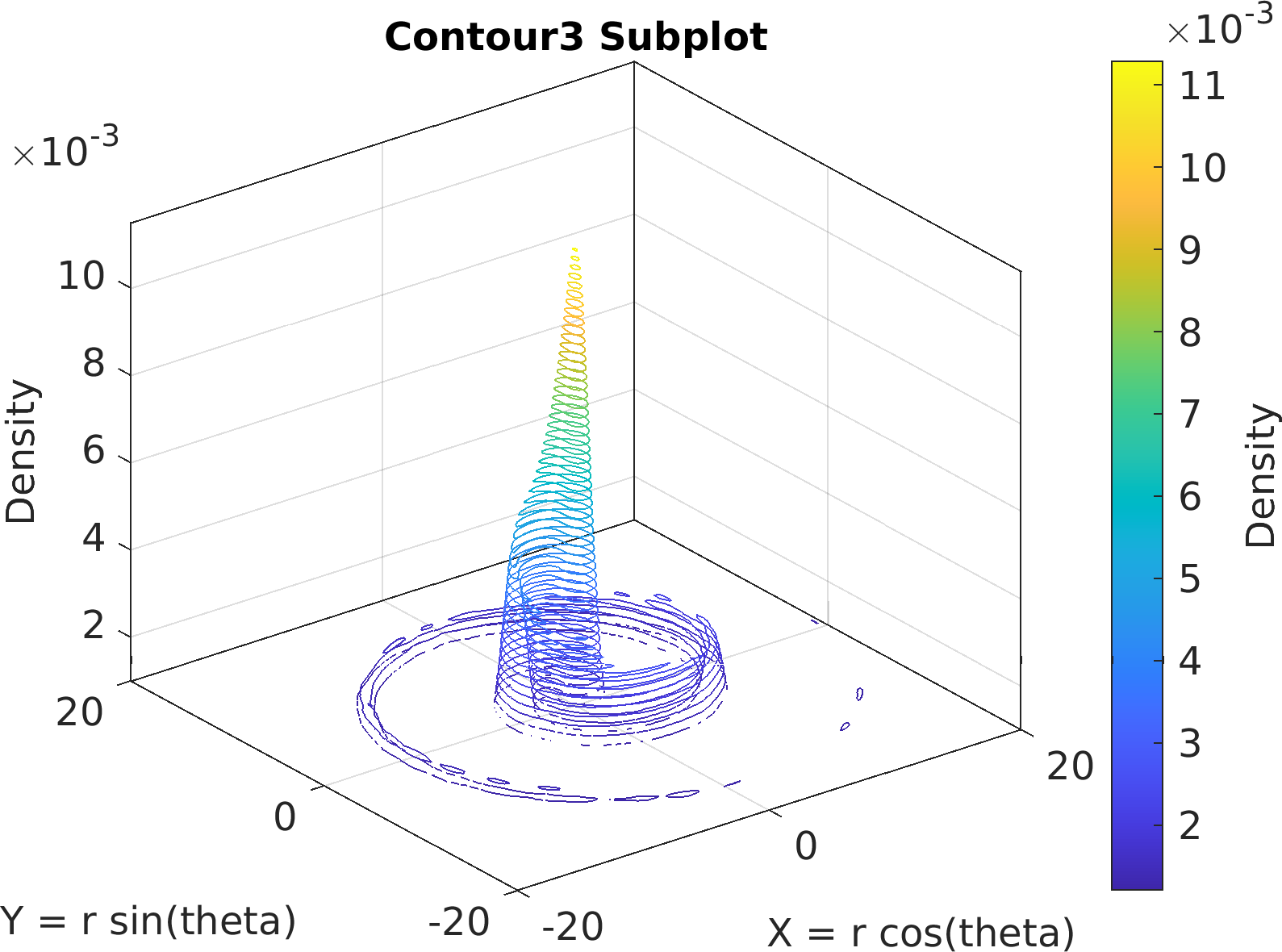
72sv = pm.vis.Subplot(
"Contour3", df);
73sv.title.titletext =
"Contour3 Subplot";
74sv.make(
"colx", 1,
"coly", 2,
"xlim", [-20, 20],
"ylim", [-20, 20]);
75pm.vis.figure.savefig(
"SubplotContour3.1.png",
"-m3");
77figure(
"color",
"white");
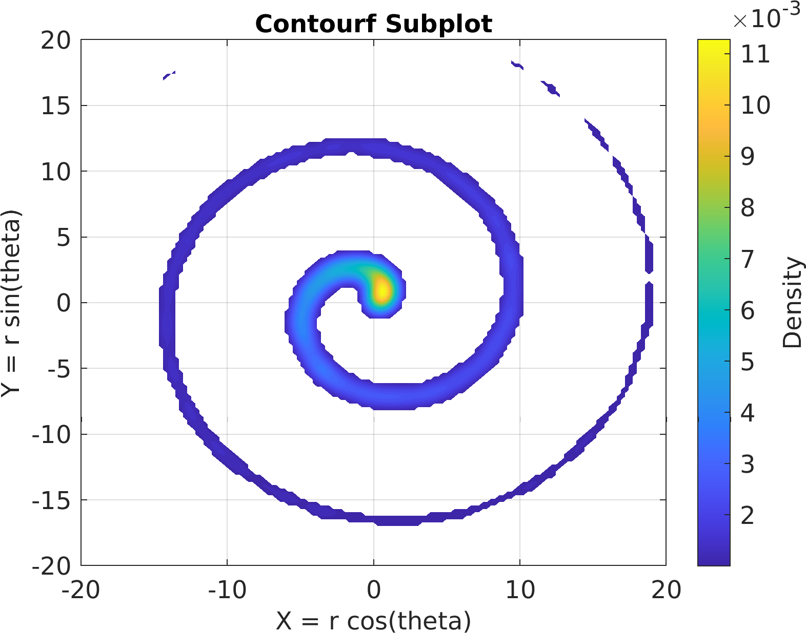
78sv = pm.vis.Subplot(
"Contourf", df);
79sv.title.titletext =
"Contourf Subplot";
80sv.make(
"colx", 1,
"coly", 2,
"xlim", [-20, 20],
"ylim", [-20, 20]);
81pm.vis.figure.savefig(
"SubplotContourf.1.png",
"-m3");
83figure(
"color",
"white");
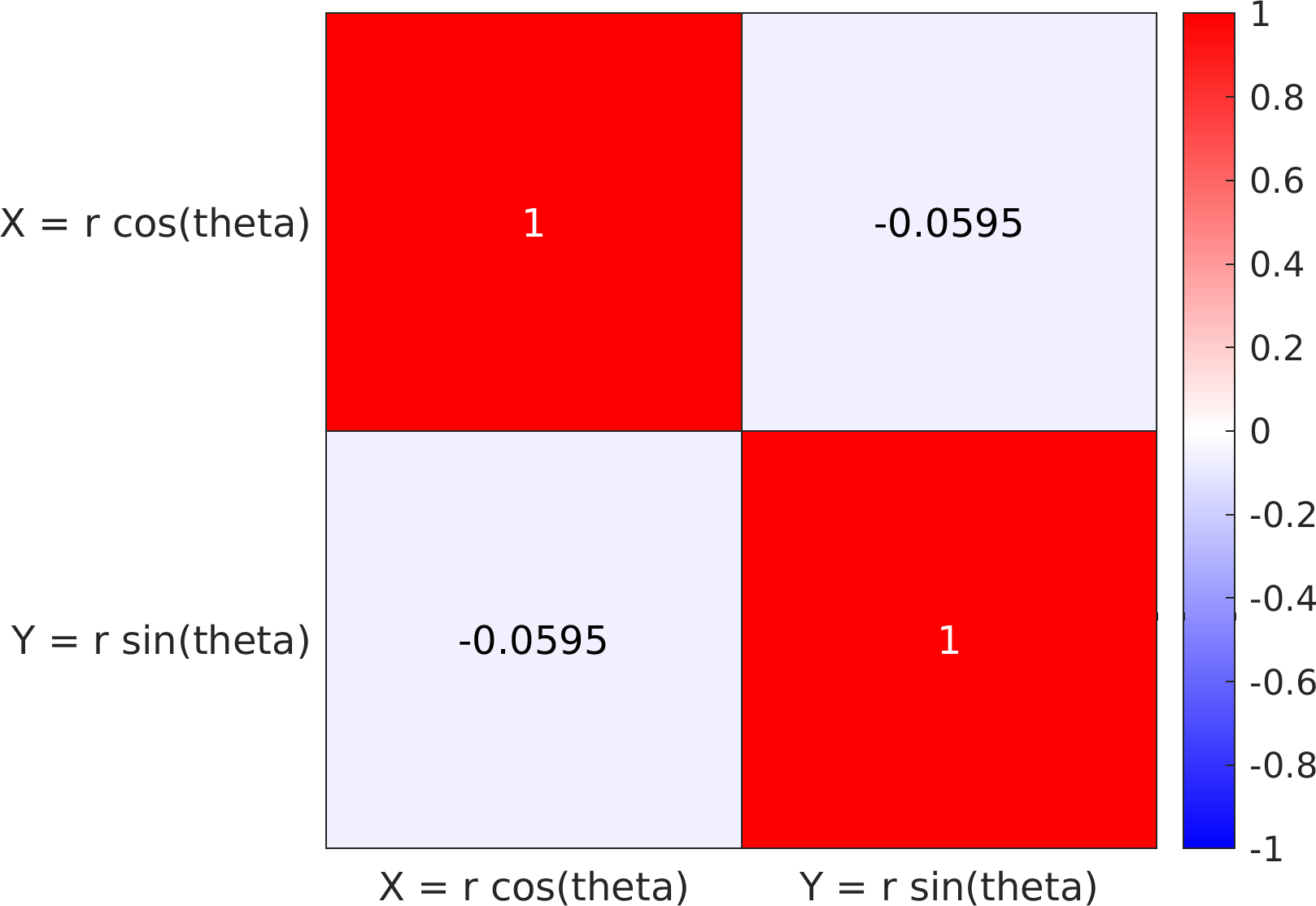
84dfcor = pm.stats.Cor(df(:, 1 : 2));
85sv = pm.vis.Subplot(
"Heatmap", dfcor.val);
87title(
"Heatmap Subplot");
88pm.vis.figure.savefig(
"SubplotHeatmap.1.png",
"-m3");
90%%%% Make Ellipse plots.
92sampler = pm.sampling.Paradram();
93sampler.spec.outputStatus =
"retry";
94sampler.spec.outputFileName =
"mvn";
95sampler.spec.randomSeed = 28457353; %
make sampling reproducible.
96sampler.spec.outputChainSize = 30000; % Use a small chain size
for illustration.
97sampler.spec.outputRestartFileFormat =
"ascii";
99sampler.run(@(x) -sum((x - [-5; 5; 10; -10]) .^ 2), 4);
100restart = sampler.readRestart();
103figure(
"color",
"white");
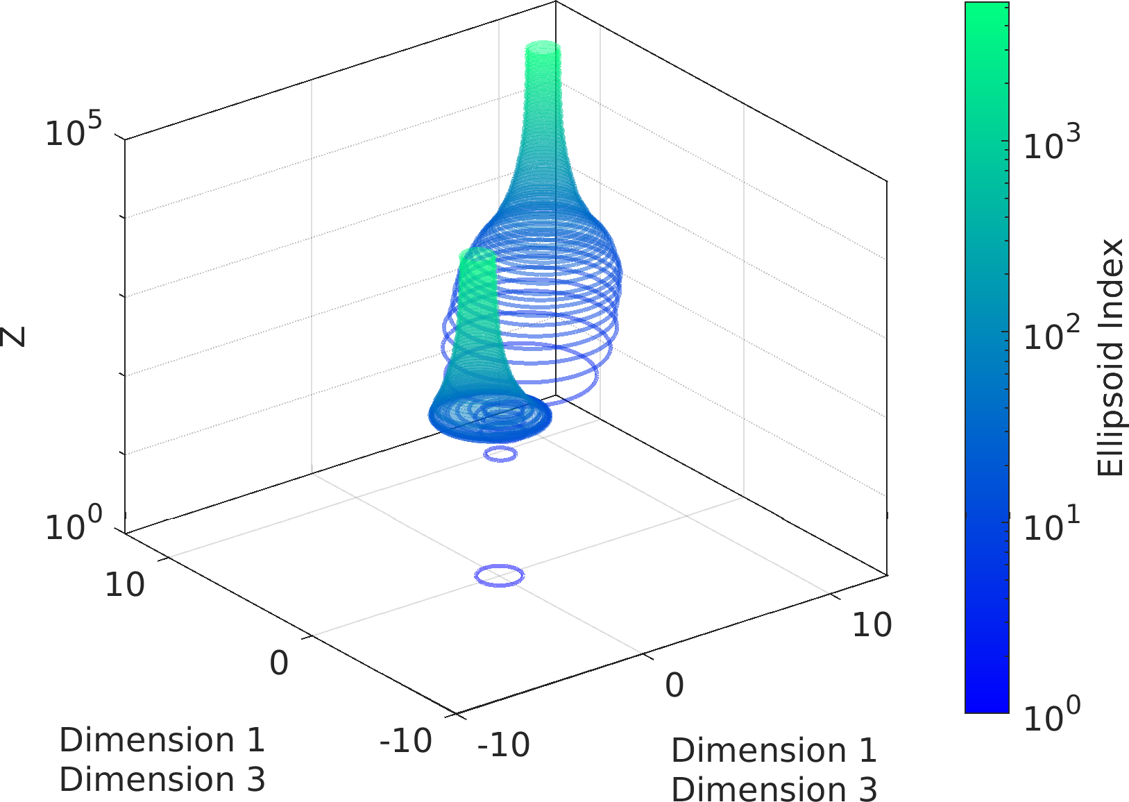
104sv = pm.vis.SubplotEllipse(restart.proposalCov, restart.proposalMean);
105pv.subplot.title.titletext =
"Ellipse Subplot";
106sv.make(
"axes", {
"zscale",
"log"},
"dimx", [1, 3],
"dimy", [1, 3] + 1);
107pm.vis.figure.savefig(
"SubplotEllipse.1.png",
"-m3");
109figure(
"color",
"white");
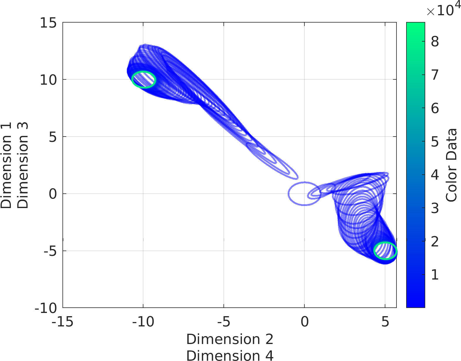
110sv = pm.vis.SubplotEllipse3(restart.proposalCov, restart.proposalMean, transpose(restart.uniqueStateVisitCount));
111pv.subplot.title.titletext =
"Ellipse3 Subplot";
112sv.make(
"axes", {
"zscale",
"log"},
"dimx", [1, 3],
"dimy", [1, 3] + 1);
113pm.vis.figure.savefig(
"SubplotEllipse3.1.png",
"-m3");
function make(in self, in varargin)
Generate a plot from the selected columns of the parent object component dfref.
function root()
Return a scalar MATLAB string containing the root directory of the ParaMonte library package.
Visualization of the example output ⛓
Final Remarks ⛓
If you believe this algorithm or its documentation can be improved, we appreciate your contribution and help to edit this page's documentation and source file on GitHub.
For details on the naming abbreviations, see this page.
For details on the naming conventions, see this page.
This software is distributed under the MIT license with additional terms outlined below.
-
If you use any parts or concepts from this library to any extent, please acknowledge the usage by citing the relevant publications of the ParaMonte library.
-
If you regenerate any parts/ideas from this library in a programming environment other than those currently supported by this ParaMonte library (i.e., other than C, C++, Fortran, MATLAB, Python, R), please also ask the end users to cite this original ParaMonte library.
This software is available to the public under a highly permissive license.
Help us justify its continued development and maintenance by acknowledging its benefit to society, distributing it, and contributing to it.
- Copyright
- Computational Data Science Lab
- Author:
- Joshua Alexander Osborne, May 22 2024, 6:45 PM, University of Texas at Arlington
Amir Shahmoradi, July 5 2024, 1:07 PM, NASA Goddard Space Flight Center (GSFC), Washington, D.C.
| function Subplot::make |
( |
in |
self, |
|
|
in |
varargin |
|
) |
| |
Generate a plot from the selected columns of the parent object component dfref.
- Parameters
-
| [in,out] | self | : The input/output parent object of class pm.vis.Subplot which is implicitly passed to this dynamic method (not by the user).
|
| [in] | varargin | : Any property, value pair of the parent object.
If the property is a struct(), then its value must be given as a cell array, with consecutive elements representing the struct property-name, property-value pairs.
Note that all of these property-value pairs can be also directly set via the parent object attributes, before calling the make() method.
|
Possible calling interfaces ⛓
s = pm.vis.Subplot(ptype,
dfref)
s.make(varargin);
s.make();
- Warning
- This method has side-effects by manipulating the existing attributes of the parent object.
Example usage ⛓
s = pm.vis.Subplot(
"scatter",
dfref);
s.make("colx", 1, "coly", 2, "colc", 3)
Example usage ⛓
1cd(fileparts(mfilename(
'fullpath'))); % Change working directory to source code directory.
2addpath(
'../../../'); % Add the ParaMonte library
root directory to the search path.
4theta = linspace(0, 8 * pi, 500);
6df = array2table(ctranspose([r .* cos(theta); r .* sin(theta); r(end) - r]));
7df.Properties.VariableNames = [
"X = r cos(theta)",
"Y = r sin(theta)",
"Z = r"];
9figure(
"color",
"white");
10sv = pm.vis.Subplot(
"Line", df);
11sv.title.titletext =
"Line Subplot";
12sv.surface.lineWidth = 2;
13sv.make(
"colx", 1,
"coly", 2);
14pm.vis.figure.savefig(
"SubplotLine.1.png",
"-m3");
16figure(
"color",
"white");
17sv = pm.vis.Subplot(
"Line3", df);
18sv.title.titletext =
"Line3 Subplot";
19sv.surface.lineWidth = 2;
20sv.make(
"colx", 1,
"coly", 2,
"colz", 3);
21pm.vis.figure.savefig(
"SubplotLine3.1.png",
"-m3");
23figure(
"color",
"white");
24sv = pm.vis.Subplot(
"Scatter", df);
25sv.title.titletext =
"Scatter Subplot";
26sv.make(
"colx", 1,
"coly", 2);
27pm.vis.figure.savefig(
"SubplotScatter.1.png",
"-m3");
29figure(
"color",
"white");
30sv = pm.vis.Subplot(
"Scatter3", df);
31sv.title.titletext =
"Scatter3 Subplot";
32sv.make(
"colx", 1,
"coly", 2,
"colz", 3);
33pm.vis.figure.savefig(
"SubplotScatter3.1.png",
"-m3");
35figure(
"color",
"white");
36sv = pm.vis.Subplot(
"LineScatter", df);
37sv.title.titletext =
"LineScatter Subplot";
38sv.make(
"colx", 1,
"coly", 2);
39pm.vis.figure.savefig(
"SubplotLineScatter.1.png",
"-m3");
41figure(
"color",
"white");
42sv = pm.vis.Subplot(
"LineScatter3", df);
43sv.title.titletext =
"LineScatter3 Subplot";
44sv.make(
"colx", 1,
"coly", 2,
"colz", 3);
45pm.vis.figure.savefig(
"SubplotLineScatter3.1.png",
"-m3");
47figure(
"color",
"white");
48sv = pm.vis.Subplot(
"Histogram", df);
49sv.title.titletext =
"Histogram Subplot";
51pm.vis.figure.savefig(
"SubplotHistogram.1.png",
"-m3");
53figure(
"color",
"white");
54sv = pm.vis.Subplot(
"Histogram2", df);
55sv.title.titletext =
"Histogram2 Subplot";
56sv.make(
"colx", 1,
"coly", 2);
57pm.vis.figure.savefig(
"SubplotHistogram2.1.png",
"-m3");
59figure(
"color",
"white");
60sv = pm.vis.Subplot(
"Histfit", df);
61sv.title.titletext =
"Histfit Subplot";
63pm.vis.figure.savefig(
"SubplotHistfit.1.png",
"-m3");
65figure(
"color",
"white");
66sv = pm.vis.Subplot(
"Contour", df);
67sv.title.titletext =
"Contour Subplot";
68sv.make(
"colx", 1,
"coly", 2,
"xlim", [-20, 20],
"ylim", [-20, 20]);
69pm.vis.figure.savefig(
"SubplotContour.1.png",
"-m3");
71figure(
"color",
"white");
72sv = pm.vis.Subplot(
"Contour3", df);
73sv.title.titletext =
"Contour3 Subplot";
74sv.make(
"colx", 1,
"coly", 2,
"xlim", [-20, 20],
"ylim", [-20, 20]);
75pm.vis.figure.savefig(
"SubplotContour3.1.png",
"-m3");
77figure(
"color",
"white");
78sv = pm.vis.Subplot(
"Contourf", df);
79sv.title.titletext =
"Contourf Subplot";
80sv.make(
"colx", 1,
"coly", 2,
"xlim", [-20, 20],
"ylim", [-20, 20]);
81pm.vis.figure.savefig(
"SubplotContourf.1.png",
"-m3");
83figure(
"color",
"white");
84dfcor = pm.stats.Cor(df(:, 1 : 2));
85sv = pm.vis.Subplot(
"Heatmap", dfcor.val);
87title(
"Heatmap Subplot");
88pm.vis.figure.savefig(
"SubplotHeatmap.1.png",
"-m3");
90%%%% Make Ellipse plots.
92sampler = pm.sampling.Paradram();
93sampler.spec.outputStatus =
"retry";
94sampler.spec.outputFileName =
"mvn";
95sampler.spec.randomSeed = 28457353; %
make sampling reproducible.
96sampler.spec.outputChainSize = 30000; % Use a small chain size
for illustration.
97sampler.spec.outputRestartFileFormat =
"ascii";
99sampler.run(@(x) -sum((x - [-5; 5; 10; -10]) .^ 2), 4);
100restart = sampler.readRestart();
103figure(
"color",
"white");
104sv = pm.vis.SubplotEllipse(restart.proposalCov, restart.proposalMean);
105pv.subplot.title.titletext =
"Ellipse Subplot";
106sv.make(
"axes", {
"zscale",
"log"},
"dimx", [1, 3],
"dimy", [1, 3] + 1);
107pm.vis.figure.savefig(
"SubplotEllipse.1.png",
"-m3");
109figure(
"color",
"white");
110sv = pm.vis.SubplotEllipse3(restart.proposalCov, restart.proposalMean, transpose(restart.uniqueStateVisitCount));
111pv.subplot.title.titletext =
"Ellipse3 Subplot";
112sv.make(
"axes", {
"zscale",
"log"},
"dimx", [1, 3],
"dimy", [1, 3] + 1);
113pm.vis.figure.savefig(
"SubplotEllipse3.1.png",
"-m3");
Visualization of the example output ⛓
Final Remarks ⛓
If you believe this algorithm or its documentation can be improved, we appreciate your contribution and help to edit this page's documentation and source file on GitHub.
For details on the naming abbreviations, see this page.
For details on the naming conventions, see this page.
This software is distributed under the MIT license with additional terms outlined below.
-
If you use any parts or concepts from this library to any extent, please acknowledge the usage by citing the relevant publications of the ParaMonte library.
-
If you regenerate any parts/ideas from this library in a programming environment other than those currently supported by this ParaMonte library (i.e., other than C, C++, Fortran, MATLAB, Python, R), please also ask the end users to cite this original ParaMonte library.
This software is available to the public under a highly permissive license.
Help us justify its continued development and maintenance by acknowledging its benefit to society, distributing it, and contributing to it.
- Copyright
- Computational Data Science Lab
- Author:
- Joshua Alexander Osborne, May 22 2024, 6:36 PM, University of Texas at Arlington
Fatemeh Bagheri, May 20 2024, 1:25 PM, NASA Goddard Space Flight Center (GSFC), Washington, D.C.
Amir Shahmoradi, July 5 2024, 1:07 PM, NASA Goddard Space Flight Center (GSFC), Washington, D.C.
| function Subplot::premake |
( |
in |
self, |
|
|
in |
varargin |
|
) |
| |
Prepare the subplot for visualization.
- Parameters
-
| [in,out] | self | : The input/output parent object of class pm.vis.Subplot which is implicitly passed to this dynamic method (not by the user).
|
| [in] | varargin | : Any property, value pair of the parent object.
If the property is a struct(), then its value must be given as a cell array, with consecutive elements representing the struct property-name, property-value pairs.
Note that all of these property-value pairs can be also directly set via the parent object attributes, before calling the premake() method.
|
Possible calling interfaces ⛓
s = pm.vis.Subplot(ptype,
dfref);
s.premake(varargin);
s.premake();
- Warning
- This method has side-effects by manipulating the existing attributes of the parent object.
Example usage ⛓
s = pm.vis.Subplot(
"scatter",
dfref);
s.premake("colx", 1, "coly", 2, "colc", 3)
Final Remarks ⛓
If you believe this algorithm or its documentation can be improved, we appreciate your contribution and help to edit this page's documentation and source file on GitHub.
For details on the naming abbreviations, see this page.
For details on the naming conventions, see this page.
This software is distributed under the MIT license with additional terms outlined below.
-
If you use any parts or concepts from this library to any extent, please acknowledge the usage by citing the relevant publications of the ParaMonte library.
-
If you regenerate any parts/ideas from this library in a programming environment other than those currently supported by this ParaMonte library (i.e., other than C, C++, Fortran, MATLAB, Python, R), please also ask the end users to cite this original ParaMonte library.
This software is available to the public under a highly permissive license.
Help us justify its continued development and maintenance by acknowledging its benefit to society, distributing it, and contributing to it.
- Copyright
- Computational Data Science Lab
- Author:
- Joshua Alexander Osborne, May 22 2024, 6:41 PM, University of Texas at Arlington
Fatemeh Bagheri, May 20 2024, 1:25 PM, NASA Goddard Space Flight Center (GSFC), Washington, D.C.
Amir Shahmoradi, July 5 2024, 1:07 PM, NASA Goddard Space Flight Center (GSFC), Washington, D.C.
| function Subplot::reset |
( |
in |
self, |
|
|
in |
varargin |
|
) |
| |
Reset the properties of the plot to the original default settings.
Use this method when you change many attributes of the plot and you want to clean up and go back to the default settings.
- Parameters
-
| [in,out] | self | : The input/output parent object of class pm.vis.Subplot which is implicitly passed to this dynamic method (not by the user).
|
| [in] | varargin | : Any property, value pair of the parent object.
If the property is a struct(), then its value must be given as a cell array, with consecutive elements representing the struct property-name, property-value pairs.
Note that all of these property-value pairs can be also directly set via the parent object attributes, before calling the make() method.
|
Possible calling interfaces ⛓
pm.vis.Subplot.reset() %
reset the plot to the
default settings.
function reset(in self, in varargin)
Reset the properties of the plot to the original default settings.
Final Remarks ⛓
If you believe this algorithm or its documentation can be improved, we appreciate your contribution and help to edit this page's documentation and source file on GitHub.
For details on the naming abbreviations, see this page.
For details on the naming conventions, see this page.
This software is distributed under the MIT license with additional terms outlined below.
-
If you use any parts or concepts from this library to any extent, please acknowledge the usage by citing the relevant publications of the ParaMonte library.
-
If you regenerate any parts/ideas from this library in a programming environment other than those currently supported by this ParaMonte library (i.e., other than C, C++, Fortran, MATLAB, Python, R), please also ask the end users to cite this original ParaMonte library.
This software is available to the public under a highly permissive license.
Help us justify its continued development and maintenance by acknowledging its benefit to society, distributing it, and contributing to it.
- Copyright
- Computational Data Science Lab
- Author:
- Joshua Alexander Osborne, May 22 2024, 6:43 PM, University of Texas at Arlington
Fatemeh Bagheri, May 20 2024, 1:25 PM, NASA Goddard Space Flight Center (GSFC), Washington, D.C.
Amir Shahmoradi, July 5 2024, 1:07 PM, NASA Goddard Space Flight Center (GSFC), Washington, D.C.