kde2d.m File Reference

Go to the source code of this file.

Functions
function	kde2d (in data, in resol, in xymin, in xymax)
	Compute the Gaussian kernel density estimate of the input bivariate data. More...

Function Documentation

kde2d()

function kde2d	(	in	data,
		in	resol,
		in	xymin,
		in	xymax
	)

Compute the Gaussian kernel density estimate of the input bivariate data.

This function offers a fast and accurate bivariate kernel density estimator with diagonal bandwidth matrix.
The kernel is assumed to be Gaussian.
The two bandwidth parameters are chosen optimally without ever using/assuming a parametric model for the data or any rules of thumb.
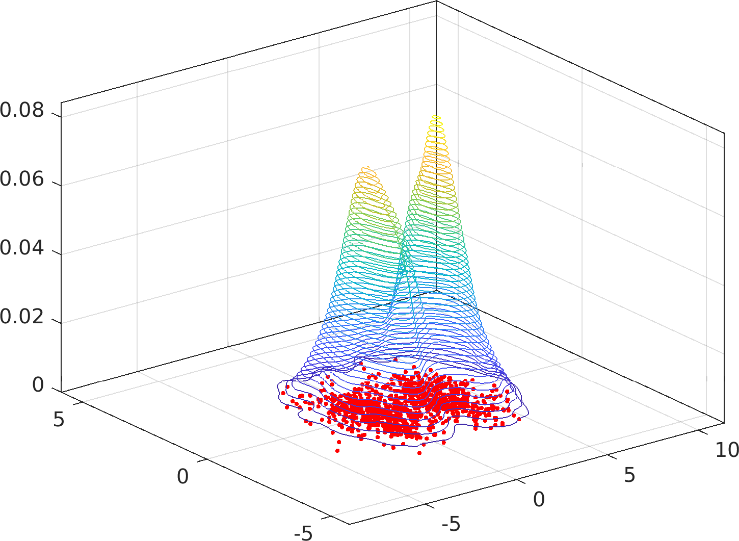
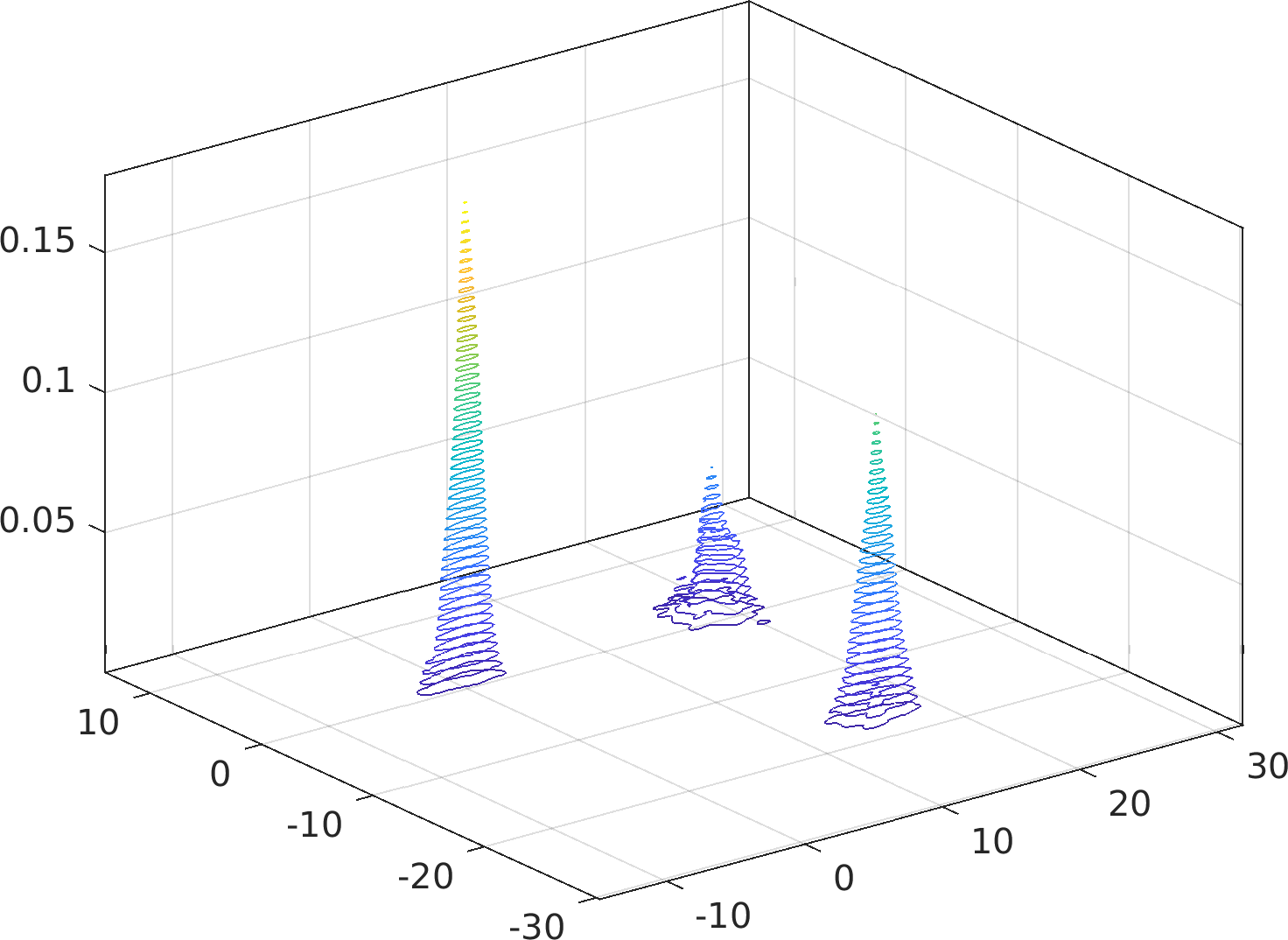
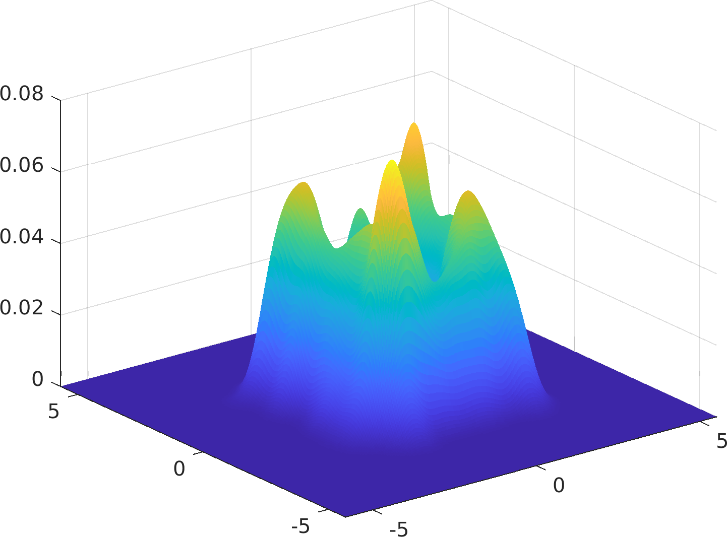
Particularly, this algorithm is immune to accuracy failures in the estimation of multimodal densities with widely separated modes (see examples below).

Parameters

[in]	data	: The input matrix of shape [nobs, 2] containing the continuous data whose density estimate is to be returned.
[in]	resol	: The input scalar whole number representing the size of the resol by resol grid over which the density is computed where resol has to be a power of 2, otherwise resol = 2 ^ ceil(log2(resol)) will be used. (optional. If missing or empty, it will be set to 2^8.)
[in]	xymin	: The input vector of size 2 containing the lower limits of the bounding box over which the density is computed. (optional. If missing or empty, it will be set to an appropriate value as prescribed in the note below.)
[in]	xymax	: The input vector of size 2 containing the upper limits of the bounding box over which the density is computed. (optional. If missing or empty, it will be set to an appropriate value as prescribed in the note below.)

Returns

bandwidth : The output row vector with the two optimal bandwidths for a bivaroate Gaussian kernel.
The format of the vector is bandwidth = [bandwidth_x, bandwidth_y].

density : The output resol by resol matrix containing the density values over the resol by resol grid.
This argument is not computed unless the output argument is present.

meshx : The x-axis meshgrid over which the variable "density" has been computed.
This output is particularly useful in combination with MATLAB intrinsic surf.
The intended usage is surf(meshx, meshy, density).

meshy : The y-axis meshgrid over which the variable "density" has been computed.
This output is particularly useful in combination with MATLAB intrinsic surf.
The intended usage is surf(meshx, meshy, density).

Possible calling interfaces ⛓

[bandwidth, density, meshx, meshy] = pm.stats.hist.kde2d(data);
[bandwidth, density, meshx, meshy] = pm.stats.hist.kde2d(data, resol);
[bandwidth, density, meshx, meshy] = pm.stats.hist.kde2d(data, resol, xymin);
[bandwidth, density, meshx, meshy] = pm.stats.hist.kde2d(data, resol, xymin, xymax);

Note

The procedure for computing the default values for the input arguments xymin and xymax are as follows:

dmax = max(data, [], 1);
dmin = min(data, [], 1);
dlim = dmax - dmin;
xymax = dmax + dlim / 4;
xymin = dmin - dlim / 4;

See also

Kernel density estimation via diffusion, Z. I. Botev, J. F. Grotowski, and D. P. Kroese (2010) Annals of Statistics, Volume 38, Number 5, pages 2916-2957.
pm.vis.SubplotContour
pm.vis.CascadeContour
pm.vis.PlotContour
pm.vis.TileContour
pm.vis.SubplotContourf
pm.vis.CascadeContourf
pm.vis.PlotContourf
pm.vis.TileContourf
pm.vis.SubplotContour3
pm.vis.CascadeContour3
pm.vis.PlotContour3
pm.vis.TileContour3

Example usage ⛓

cd(fileparts(mfilename('fullpath'))); % Change working directory to source code directory.
addpath('../../../../../'); % Add the ParaMonte library root directory to the search path.
 
%%%%
%%%% Generate a Gaussian mixture with distant modes.
%%%%
 
data = [ randn(500, 2) ...
       ; randn(500, 1) + 3.5, randn(500, 1) ...
       ];
 
[bandwidth, density, meshx, meshy] = pm.stats.hist.kde2d(data);
 
% Plot the data and the density estimate.
figure("color", "white");
contour3(meshx, meshy, density, 50); hold on;
plot(data(:, 1), data(:, 2), 'r.', 'MarkerSize', 5);
pm.vis.figure.savefig("pm.stats.hist.kde2d.mvnmix.png", "-m3");

Visualization of the example output ⛓

Example usage ⛓

cd(fileparts(mfilename('fullpath'))); % Change working directory to source code directory.
addpath('../../../../../'); % Add the ParaMonte library root directory to the search path.
 
%%%%
%%%% Generate a Gaussian mixture with distant modes.
%%%%
 
data =  [ randn(100, 1), randn(100, 1) / 4 ...
        ; randn(100, 1) + 18, randn(100,1) ...
        ; randn(100, 1) + 15, randn(100, 1)/ 2 - 18 ...
        ];
 
[bandwidth, density, meshx, meshy] = pm.stats.hist.kde2d(data);
 
% Plot the data and the density estimate.
figure("color", "white");
contour3(meshx, meshy, density, 50);
%colormap("hot"); hold on; alpha(.8); view([0, 60]);
%plot(data(:, 1), data(:, 2), 'w.', 'MarkerSize', 5);
pm.vis.figure.savefig("pm.stats.hist.kde2d.mvnmixfar.png", "-m3");

Visualization of the example output ⛓

Example usage ⛓

cd(fileparts(mfilename('fullpath'))); % Change working directory to source code directory.
addpath('../../../../../'); % Add the ParaMonte library root directory to the search path.
 
%%%%
%%%% Generate a Sinusoidal density.
%%%%
 
resol = 1000;
meshx = 2 * cos(rand(resol, 1) * 10 * pi) + randn(resol, 1) / 3;%rand(1000, 1); 
meshy = 2 * sin(rand(resol, 1) * 10 * pi) + randn(resol, 1) / 3;
data = [meshx, meshy];
 
[bandwidth, density, meshx, meshy] = pm.stats.hist.kde2d(data);
 
% Plot the data and the density estimate.
figure("color", "white");
surf(meshx, meshy, density, 'LineStyle', 'none'); 
%colorbar();
%view([0, 70]); hold on; alpha(.8);
%plot(data(:, 1), data(:, 2), 'w.', 'MarkerSize', 5);
pm.vis.figure.savefig("pm.stats.hist.kde2d.sincos.png", "-m3");

Visualization of the example output ⛓

Final Remarks ⛓

---

If you believe this algorithm or its documentation can be improved, we appreciate your contribution and help to edit this page's documentation and source file on GitHub.
For details on the naming abbreviations, see this page.
For details on the naming conventions, see this page.
This software is distributed under the MIT license with additional terms outlined below.

1. If you use any parts or concepts from this library to any extent, please acknowledge the usage by citing the relevant publications of the ParaMonte library.
   
2. If you regenerate any parts/ideas from this library in a programming environment other than those currently supported by this ParaMonte library (i.e., other than C, C++, Fortran, MATLAB, Python, R), please also ask the end users to cite this original ParaMonte library.
   

This software is available to the public under a highly permissive license.
Help us justify its continued development and maintenance by acknowledging its benefit to society, distributing it, and contributing to it.

Copyright

Computational Data Science Lab

Copyright (c) 2015, Dr. Zdravko Botev All rights reserved.

Redistribution and use in source and binary forms, with or without modification, are permitted provided that the following conditions are met:

• Redistributions of source code must retain the above copyright notice, this list of conditions and the following disclaimer.
• Redistributions in binary form must reproduce the above copyright notice, this list of conditions and the following disclaimer in the documentation and/or other materials provided with the distribution
• Neither the name of the The University of New South Wales nor the names of its contributors may be used to endorse or promote products derived from this software without specific prior written permission.

This software is provided by the copyright holders and contributors "as is" and any express or implied warranties, including, but not limited to, the implied warranties of merchantability and fitness for a particular purpose are disclaimed. In no event shall the copyright owner or contributors be liable for any direct, indirect, incidental, special, exemplary, or consequential damages (including, but not limited to, procurement of substitute goods or services; loss of use, data, or profits; or business interruption) however caused and on any theory of liability, whether in contract, strict liability, or tort (including negligence or otherwise) arising in any way out of the use of this software, even if advised of the possibility of such damage.

Amir Shahmoradi, May 16 2016, 9:03 AM, Oden Institute for Computational Engineering and Sciences (ICES), UT Austin