getLogUDF.m File Reference

Go to the source code of this file.

Functions
function	getLogUDF (in x, in y, in epsilon)
	Return the natural logarithm of the Unnormalized Density Function (UDF) of the inverse of the 2-dimensional modified Himmelblau function. More...

Function Documentation

getLogUDF()

function getLogUDF	(	in	x,
		in	y,
		in	epsilon
	)

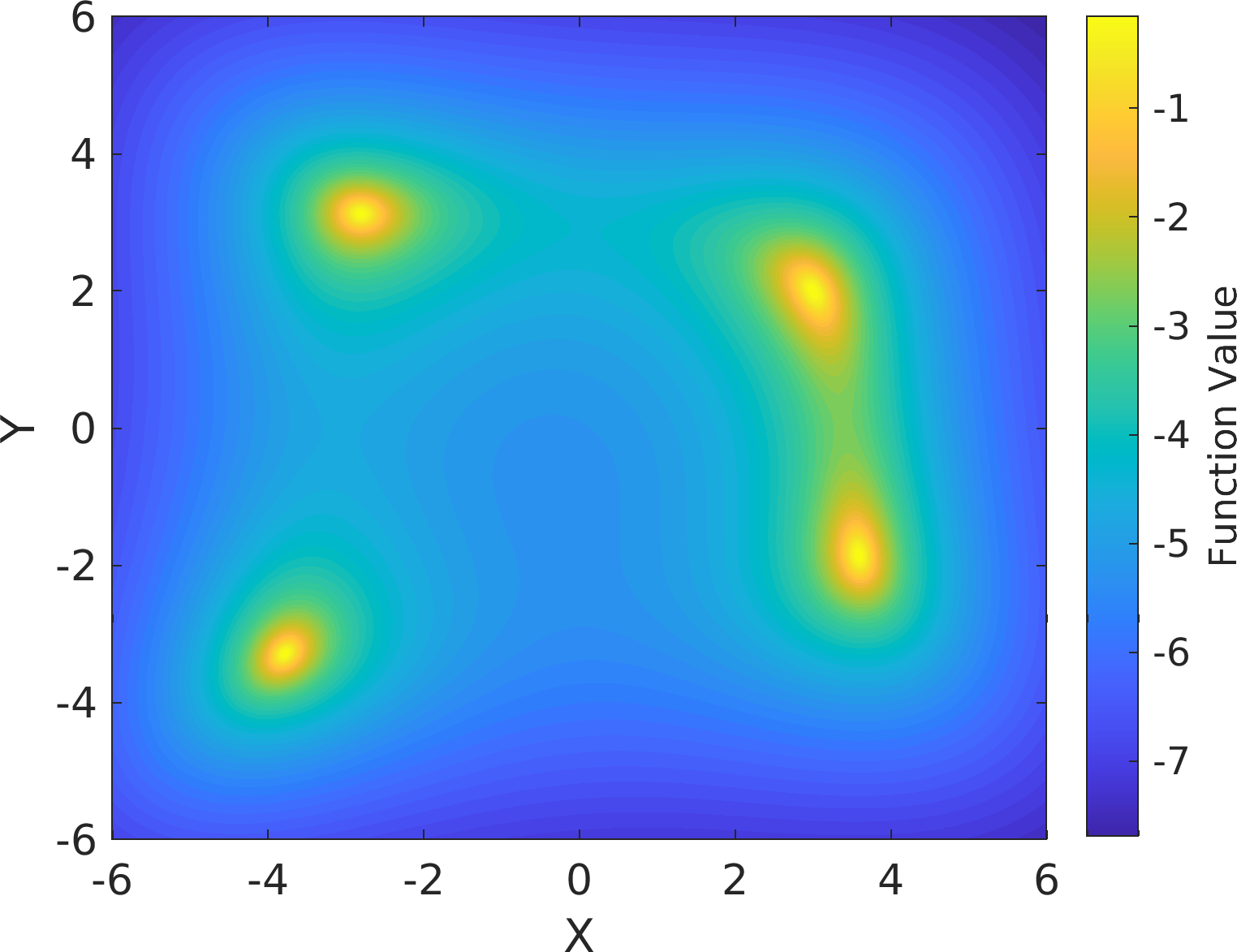
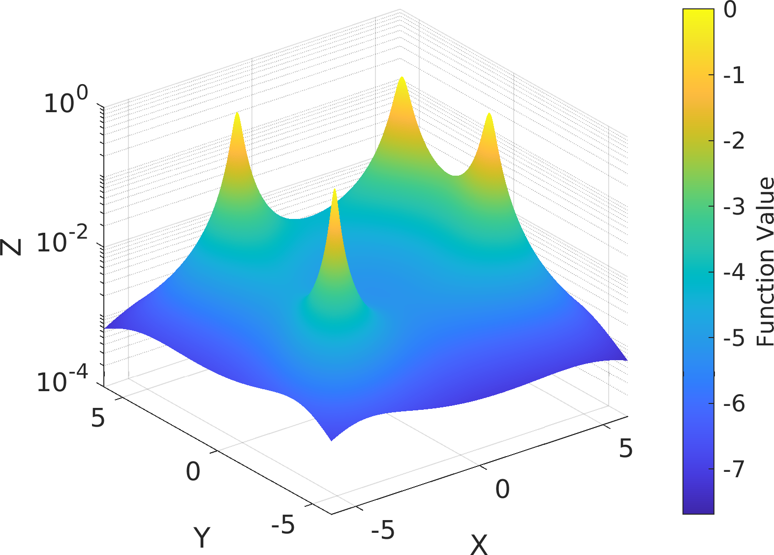
Return the natural logarithm of the Unnormalized Density Function (UDF) of the inverse of the 2-dimensional modified Himmelblau function.

Himmelblau's function is a multi-modal function, used to test the performance of optimization algorithms. The function is defined by:

\begin{equation} H(x, y) = (x^{2} + y - 11)^{2} + (x + y^{2} - 7)^{2} ~. \end{equation}

It has one local maximum at \(x = -0.270845\) and \(y = -0.923039\) where \(H(x, y) = 181.617\), and four identical local minima:

\begin{eqnarray} H(3.0,2.0) &=& 0.0 ~,\\ H(-2.805118, 3.131312) &=& 0.0 ~,\\ H(-3.779310, -3.283186) &=& 0.0 ~,\\ H(3.584428, -1.848126) &=& 0.0 ~. \end{eqnarray}

The function is named after David Mautner Himmelblau (1924–2011), who introduced it.
The locations of all the minima can be found analytically.

This MATLAB function returns a modification of the Himmelblau function as a density function suitable for testing sampling algorithms (or stochastic maximizers):

\begin{equation} f(x, y, \epsilon) = \frac{1}{H(x, y) + \epsilon} ~. \end{equation}

where \(\epsilon\) is an arbitrary positive real number which determines the sharpness of the function four peaks.

Parameters

[in]	x	: The input scalar or array of the same rank and shape as other input array-like arguments of type MATLAB double, representing the x-component of the state within the domain of Himmelblau density at which the density value must be computed.
[in]	y	: The input scalar or array of the same rank and shape as other input array-like arguments of type MATLAB double, representing the y-component of the state within the domain of Himmelblau density at which the density value must be computed.
[in]	epsilon	: The input positive scalar or array of the same rank and shape as other array-like input arguments of type MATLAB double, representing the value to be added to the inverse of the Himmelblau function. Increasingly smaller values of epsilon will yield pointier densities. Increasingly larger values of epsilon will yield flatter densities. (optional, default = 1)

Returns

logUDF : The output Unnormalized Density Function (UDF) of the Himmelblau density at the specified input state.

Possible calling interfaces ⛓

logUDF = pm.stats.himmelblau.getLogUDF(state);
logUDF = pm.stats.himmelblau.getLogUDF(state, epsilon);

See also

pm.stats.himmelblau.getFunc
pm.stats.himmelblau.getLogUDF
pm.sampling.Paradram

Example usage ⛓

cd(fileparts(mfilename('fullpath'))); % Change working directory to source code directory.
addpath('../../../../../'); % Add the ParaMonte library root directory to the search path.
 
range = -6 : 0.01 : 6;
[x, y] = meshgrid(range, range);
z = exp(pm.stats.dist.himmelblau.getLogUDF(x, y, 1));
for dim = 2 : 3
    figure("color", "white");
    if  dim == 2
        contourf(x, y, log(z), 50, "EdgeColor", "none");
    else
        surf(x, y, z, log(z), "EdgeColor", "none");
        set(gca, "zscale", "log");
        zlabel("Z");
    end
    xlabel("X");
    ylabel("Y");
    cbar = colorbar();
    ylabel(cbar, "Function Value")
    set(gca, "fontsize", 13);
    pm.vis.figure.savefig("himmelblau.getLogUDF." + string(dim) + "d.png", "-m3");
end

Visualization of the example output ⛓

Final Remarks ⛓

---

If you believe this algorithm or its documentation can be improved, we appreciate your contribution and help to edit this page's documentation and source file on GitHub.
For details on the naming abbreviations, see this page.
For details on the naming conventions, see this page.
This software is distributed under the MIT license with additional terms outlined below.

1. If you use any parts or concepts from this library to any extent, please acknowledge the usage by citing the relevant publications of the ParaMonte library.
   
2. If you regenerate any parts/ideas from this library in a programming environment other than those currently supported by this ParaMonte library (i.e., other than C, C++, Fortran, MATLAB, Python, R), please also ask the end users to cite this original ParaMonte library.
   

This software is available to the public under a highly permissive license.
Help us justify its continued development and maintenance by acknowledging its benefit to society, distributing it, and contributing to it.

Copyright

Computational Data Science Lab

Author:

Amir Shahmoradi, May 16 2016, 9:03 AM, Oden Institute for Computational Engineering and Sciences (ICES), UT Austin