pm_sampleCov Module Reference

This module contains classes and procedures for computing the properties related to the covariance matrices of a random sample. More...

Data Types
interface	getCov
	Generate and return the (optionally unbiased) covariance matrix of a pair of (potentially weighted) time series x(1:nsam) and y(1:nsam) or of an input (potentially weighted) array of shape (ndim, nsam) or (nsam, ndim) where ndim is the number of data dimensions (the number of data attributes) and nsam is the number of data points. More...
interface	getCovMerged
	Generate and return the merged covariance of a sample resulting from the merger of two separate (potentially weighted) samples \(A\) and \(B\). More...
interface	setCov
	Return the covariance matrix corresponding to the input (potentially weighted) correlation matrix or return the biased sample covariance matrix of the input array of shape (ndim, nsam) or (nsam, ndim) or a pair of (potentially weighted) time series x(1:nsam) and y(1:nsam) where ndim is the number of data dimensions (the number of data attributes) and nsam is the number of data points. More...
interface	setCovMean
	Return the covariance matrix and mean vector corresponding to the input (potentially weighted) input sample of shape (ndim, nsam) or (nsam, ndim) or a pair of (potentially weighted) time series x(1:nsam) and y(1:nsam) where ndim is the number of data dimensions (the number of data attributes) and nsam is the number of data points. More...
interface	setCovMeanMerged
	Return the merged covariance and mean of a sample resulting from the merger of two separate (potentially weighted) samples \(A\) and \(B\). More...
interface	setCovMeanUpdated
	Return the covariance and mean of a sample that results from the merger of two separate (potentially weighted) non-singular \(A\) and singular \(B\) samples. More...
interface	setCovMerged
	Return the merged covariance of a sample resulting from the merger of two separate (potentially weighted) samples \(A\) and \(B\). More...
interface	setCovUpdated
	Return the covAariance resulting from the merger of two separate (potentially weighted) non-singular and singular samples \(A\) and \(B\). More...

Variables
character(*, SK), parameter	MODULE_NAME = "@pm_sampleCov"

Detailed Description

This module contains classes and procedures for computing the properties related to the covariance matrices of a random sample.

Covariance

The concept of variance can be generalized to measure the covariation of any pair of data attributes.
The sample covariance matrix is a \(K\)-by- \(K\) matrix \(\mathbf{Q} = \left[\tilde\Sigma_{jk}\right]\) with entries,

\begin{equation} \tilde\Sigma_{jk} = \frac{1}{n} \sum_{i=1}^{n} \left( x_{ij} - \hat\mu_j \right) \left( x_{ik} - \hat\mu_k \right) ~, \end{equation}

where \(n\) is the number of observations in the sample, \(\hat\mu\) is the sample mean vector, and \(\Sigma_{jk}\) is an estimate of the covariance between the \(j\)th variable and the kth variable of the population underlying the data.

The diagonal elements of the matrix \(\tilde\Sigma_{jj}\) are known as the sample variance.

Biased sample covariance

The above formula yields a biased estimate of the covariance matrix of the sample.
Intuitively, the sample covariance relies on the difference between each observation and the sample mean, but the sample mean is slightly correlated with each observation since it is defined in terms of all observations.
Therefore, unless the sample mean is known a priori, the above equation yields a biased estimate of the covariance with sample mean as a proxy for the true mean of the population.
Note that the bias is noticeable only when the sample size is small (e.g., \(<10\)).

Unbiased sample covariance

A popular fix to the definition of sample covariance to remove its bias is to apply the Bessel correction to the equation above, yielding the unbiased covariance estimate as,

\begin{eqnarray} \hat\Sigma_{jk} &=& \frac{\xi}{n} \sum_{i=1}^{n} \left( x_{ij} - \hat\mu_j \right) \left( x_{ik} - \hat\mu_k \right) ~, &=& \frac{1}{n - 1} \sum_{i=1}^{n} \left( x_{ij} - \hat\mu_j \right) \left( x_{ik} - \hat\mu_k \right) ~, \end{eqnarray}

where \(\xi = \frac{n}{n - 1}\) is the Bessel bias correction factor.

Biased weighted sample covariance

\begin{equation} \tilde{\Sigma}^w_{jk} = \frac{ \sum_{i = 1}^{n} \left( x_{ij} - \hat\mu^w_j \right) \left( x_{ik} - \hat\mu^w_k \right) } { \left( \sum_{i=1}^{n} w_i \right) } ~. \end{equation}

where n = nsam is the number of observations in the sample, \(w_i\) are the weights of individual data points, the superscript \(^w\) signifies the sample weights, and \(\hat\mu^w\) is the weighted mean of the sample.
When the sample size is small, the above equation yields a biased estimate of the covariance.

Unbiased weighted sample covariance

There is no unique generic equation for the unbiased covariance of a weighted sample.
However, depending on the types of the weights involved, a few popular definitions exist.

1. The unbiased covariance of a sample with frequency, count, or repeat weights can be computed via the following equation,

   \begin{equation} \hat\Sigma^w_{jk} = \frac{ \sum_{i = 1}^{n} \left( x_{ij} - \hat\mu^w_j \right) \left( x_{ik} - \hat\mu^w_k \right) } { \left( \sum_{i=1}^{n} w_i \right) - 1} ~. \end{equation}

   Frequency weights represent the number of duplications of each observation in the sample whose population covariance is to be estimated.
   Therefore, the frequency weights are expected to be integers or whole numbers.
   
2. The unbiased covariance of a sample with reliability weights, also sometimes confusingly known as probability weights or importance weights, can be computed by the following equation,

   \begin{equation} \hat\Sigma^w_{jk} = \frac{ \sum_{i=1}^{n} w_i } { \left( \sum_{i=1}^{n} w_i \right)^2 - \left( \sum_{i=1}^{n} w_i^2 \right) } \sum_{i = 1}^{n} \left( x_{ij} - \hat\mu^w_j \right) \left( x_{ik} - \hat\mu^w_k \right) ~. \end{equation}

   1. Reliability weights weights, also known as reliability weights or sampling weights represent the probability of a case (or subject) being selected into the sample from a population.
      
   2. Application of the term unbiased to the above equation is controversial as some believe that bias cannot be correct without the knowledge of the sample size, which is lost in normalized weights.
      
   3. Reliability weights are frequently (but not necessarily) normalized, meaning that \(\sum^{i = 1}_{n} w_i = 1\).
      

Covariance matrix vs. correlation matrix

The covariance matrix \(\Sigma\) is related to the correlation matrix \(\rho\) by the following equation,

\begin{equation} \Sigma_{ij} = \rho_{ij} \times \sigma_{i} \times \sigma_{j} ~, \end{equation}

where \(\Sigma\) represents the covariance matrix, \(\rho\) represents the correlation matrix, and \(\sigma\) represents the standard deviations.

See also

pm_sampling
pm_sampleACT
pm_sampleCCF
pm_sampleCor
pm_sampleCov
pm_sampleConv
pm_sampleECDF
pm_sampleMean
pm_sampleNorm
pm_sampleQuan
pm_sampleScale
pm_sampleShift
pm_sampleWeight
pm_sampleAffinity
pm_sampleVar
Box and Tiao, 1973, Bayesian Inference in Statistical Analysis, Page 421.
Updating mean and variance estimates: an improved method, D.H.D. West, 1979.
Geisser and Cornfield, 1963, Posterior distributions for multivariate normal parameters.

Benchmarks:

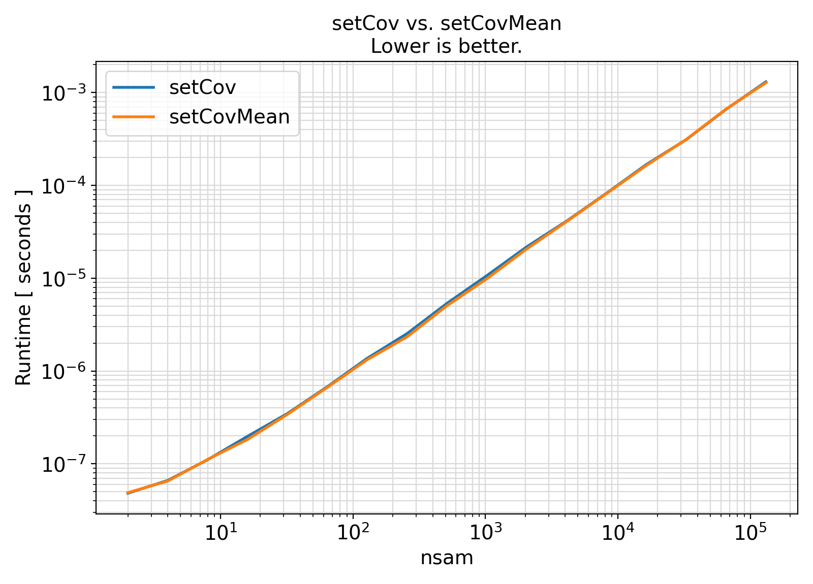
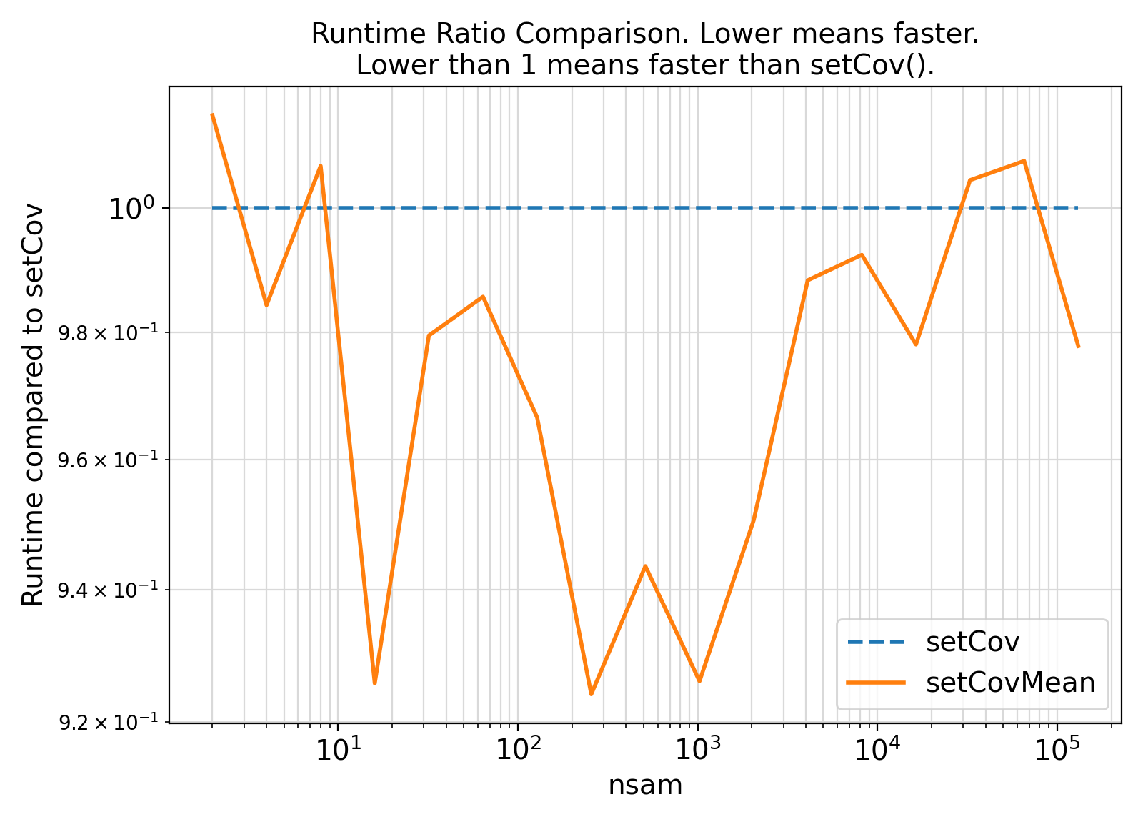
Benchmark :: The runtime performance of setCov vs. setCovMean. ⛓

! Test the performance of Cholesky factorization computation using an assumed-shape interface vs. explicit-shape interface.
program benchmark
 
    use pm_kind, only: IK, LK, RKG => RKD, SK
    use pm_sampleCov, only: uppDia
    use pm_bench, only: bench_type
 
    implicit none
 
    integer(IK)                         :: itry, ntry
    integer(IK)                         :: i
    integer(IK)                         :: iarr
    integer(IK)                         :: fileUnit
    integer(IK)     , parameter         :: NARR = 18_IK
    real(RKG)       , allocatable       :: sample(:,:)
    type(bench_type), allocatable       :: bench(:)
    integer(IK)     , parameter         :: nsammax = 2**NARR
    integer(IK)     , parameter         :: ndim = 5_IK, dim = 2
    real(RKG)                           :: mean(ndim), cov(ndim,ndim)
    integer(IK)                         :: nsam
    real(RKG)                           :: dumm
 
    bench = [ bench_type(name = SK_"setCov", exec = setCov, overhead = setOverhead) &
            , bench_type(name = SK_"setCovMean", exec = setCovMean, overhead = setOverhead) &
            ]
 
    write(*,"(*(g0,:,' '))")
    write(*,"(*(g0,:,' '))") "sample covariance benchmarking..."
    write(*,"(*(g0,:,' '))")
 
    open(newunit = fileUnit, file = "main.out", status = "replace")
 
        write(fileUnit, "(*(g0,:,','))") "nsam", (bench(i)%name, i = 1, size(bench))
 
        dumm = 0._RKG
        loopOverMatrixSize: do iarr = 1, NARR - 1
 
            nsam = 2**iarr
            ntry = nsammax / nsam
            allocate(sample(ndim, nsam))
            write(*,"(*(g0,:,' '))") "Benchmarking setCov() vs. setCovMean()", nsam, ntry
 
            do i = 1, size(bench)
                bench(i)%timing = bench(i)%getTiming()
            end do
 
            write(fileUnit,"(*(g0,:,','))") nsam, (bench(i)%timing%mean / ntry, i = 1, size(bench))
            deallocate(sample)
 
        end do loopOverMatrixSize
        write(*,"(*(g0,:,' '))") dumm
 
    close(fileUnit)
 
contains
 
    !%%%%%%%%%%%%%%%%%%%%%%%%%%%%%%%%%%%%%%%%%%%%%%%%%%%%%%%%%%%%%%%%%%%%%%%%%%%%%%%%%%%%%%%%%%%%%%%%%%%%%%%%%%%%%%%%%%%%%%%%%%%%%%%
    ! procedure wrappers.
    !%%%%%%%%%%%%%%%%%%%%%%%%%%%%%%%%%%%%%%%%%%%%%%%%%%%%%%%%%%%%%%%%%%%%%%%%%%%%%%%%%%%%%%%%%%%%%%%%%%%%%%%%%%%%%%%%%%%%%%%%%%%%%%%
 
    subroutine setOverhead()
        do itry = 1, ntry
            call setSample()
        end do
    end subroutine
 
    subroutine setSample()
        integer(IK) :: i
        call random_number(sample)
    end subroutine
 
    subroutine setCov()
        block
            use pm_sampleCov, only: setCov
            use pm_sampleMean, only: setMean
            do itry = 1, ntry
                call setSample()
                call setMean(mean, sample, dim)
                call setCov(cov, uppDia, mean, sample, dim)
                dumm = dumm + cov(1,1) - mean(ndim)
            end do
        end block
    end subroutine
 
    subroutine setCovMean()
        block
            use pm_sampleCov, only: setCovMean
            do itry = 1, ntry
                call setSample()
                call setCovMean(cov, uppDia, mean, sample, dim, sample(1:ndim, 1))
                dumm = dumm + cov(1,1) - mean(ndim)
            end do
        end block
    end subroutine
 
end program benchmark

Example Unix compile command via Intel ifort compiler ⛓

#!/usr/bin/env sh
rm main.exe
ifort -fpp -standard-semantics -O3 -Wl,-rpath,../../../lib -I../../../inc main.F90 ../../../lib/libparamonte* -o main.exe
./main.exe

Example Windows Batch compile command via Intel ifort compiler ⛓

del main.exe
set PATH=..\..\..\lib;%PATH%
ifort /fpp /standard-semantics /O3 /I:..\..\..\include main.F90 ..\..\..\lib\libparamonte*.lib /exe:main.exe
main.exe

Example Unix / MinGW compile command via GNU gfortran compiler ⛓

#!/usr/bin/env sh
rm main.exe
gfortran -cpp -ffree-line-length-none -O3 -Wl,-rpath,../../../lib -I../../../inc main.F90 ../../../lib/libparamonte* -o main.exe
./main.exe

Postprocessing of the benchmark output ⛓

#!/usr/bin/env python
 
import matplotlib.pyplot as plt
import pandas as pd
import numpy as np
 
import os
dirname = os.path.basename(os.getcwd()) 
 
fontsize = 14
 
df = pd.read_csv("main.out", delimiter = ",")
colnames = list(df.columns.values)
 
 
 
ax = plt.figure(figsize = 1.25 * np.array([6.4,4.6]), dpi = 200)
ax = plt.subplot()
 
for colname in colnames[1:]:
    plt.plot( df[colnames[0]].values
            , df[colname].values
            , linewidth = 2
            )
 
plt.xticks(fontsize = fontsize)
plt.yticks(fontsize = fontsize)
ax.set_xlabel(colnames[0], fontsize = fontsize)
ax.set_ylabel("Runtime [ seconds ]", fontsize = fontsize)
ax.set_title(" vs. ".join(colnames[1:])+"\nLower is better.", fontsize = fontsize)
ax.set_xscale("log")
ax.set_yscale("log")
plt.minorticks_on()
plt.grid(visible = True, which = "both", axis = "both", color = "0.85", linestyle = "-")
ax.tick_params(axis = "y", which = "minor")
ax.tick_params(axis = "x", which = "minor")
ax.legend   ( colnames[1:]
           #, loc='center left'
           #, bbox_to_anchor=(1, 0.5)
            , fontsize = fontsize
            )
 
plt.tight_layout()
plt.savefig("benchmark." + dirname + ".runtime.png")
 
 
 
ax = plt.figure(figsize = 1.25 * np.array([6.4,4.6]), dpi = 200)
ax = plt.subplot()
 
plt.plot( df[colnames[0]].values
        , np.ones(len(df[colnames[0]].values))
        , linestyle = "--"
       #, color = "black"
        , linewidth = 2
        )
for colname in colnames[2:]:
    plt.plot( df[colnames[0]].values
            , df[colname].values / df[colnames[1]].values
            , linewidth = 2
            )
 
plt.xticks(fontsize = fontsize)
plt.yticks(fontsize = fontsize)
ax.set_xlabel(colnames[0], fontsize = fontsize)
ax.set_ylabel("Runtime compared to {}".format(colnames[1]), fontsize = fontsize)
ax.set_title("Runtime Ratio Comparison. Lower means faster.\nLower than 1 means faster than {}().".format(colnames[1]), fontsize = fontsize)
ax.set_xscale("log")
ax.set_yscale("log")
plt.minorticks_on()
plt.grid(visible = True, which = "both", axis = "both", color = "0.85", linestyle = "-")
ax.tick_params(axis = "y", which = "minor")
ax.tick_params(axis = "x", which = "minor")
ax.legend   ( colnames[1:]
           #, bbox_to_anchor = (1, 0.5)
           #, loc = "center left"
            , fontsize = fontsize
            )
 
plt.tight_layout()
plt.savefig("benchmark." + dirname + ".runtime.ratio.png")

Visualization of the benchmark output ⛓

Benchmark moral ⛓

1. The procedures under the generic interface setCov take the sample mean as input and return the covariance matrix.
   
2. The procedures under the generic interface setCovMean compute both the sample mean and covariance matrix in one pass.
   
3. The performance of the two methods appears to depend significantly on the compiler used.
   
4. But in general, the one-pass algorithm of setCovMean appears to perform equally or slightly better than the two-pass algorithm of setCov.
   

Test:

test_pm_sampleCov

Bug:

Status: See Unresolved, See this page for more information.

Source: GNU Fortran Compiler gfortran
Description: Ideally, there should be only one generic interface in this module for computing the biased/corrected/weighted variance.
This requires ability to resolve the different weight types, which requires custom derived types for weights.
Fortran PDTs are ideal for such use cases. However, the implementation of PDTs is far from complete in GNU Fortran Compiler gfortran.

Remedy (as of ParaMonte Library version 2.0.0): Given that the importance of GNU Fortran Compiler gfortran support, separate generic interfaces were instead developed for different sample weight types.
Once the GNU Fortran Compiler gfortran PDT bugs are resolved, the getVar generic interface can be extended to serve as a high-level wrapper for the weight-specific generic interfaces in this module.

Todo:

Normal Priority: The inclusion of bias correction in the calculation of covariance is a frequentist abomination and shenanigan that must be eliminated in the future.
The correction factor should be computed separately from the actual covariance calculation.

Final Remarks ⛓

---

If you believe this algorithm or its documentation can be improved, we appreciate your contribution and help to edit this page's documentation and source file on GitHub.
For details on the naming abbreviations, see this page.
For details on the naming conventions, see this page.
This software is distributed under the MIT license with additional terms outlined below.

1. If you use any parts or concepts from this library to any extent, please acknowledge the usage by citing the relevant publications of the ParaMonte library.
   
2. If you regenerate any parts/ideas from this library in a programming environment other than those currently supported by this ParaMonte library (i.e., other than C, C++, Fortran, MATLAB, Python, R), please also ask the end users to cite this original ParaMonte library.
   

This software is available to the public under a highly permissive license.
Help us justify its continued development and maintenance by acknowledging its benefit to society, distributing it, and contributing to it.

Copyright

Computational Data Science Lab

Author:

Amir Shahmoradi, Nov 24, 2020, 4:19 AM, Dallas, TX
Fatemeh Bagheri, Thursday 12:45 AM, August 20, 2021, Dallas, TX
Amir Shahmoradi, Monday March 6, 2017, 2:48 AM, Institute for Computational Engineering and Sciences (ICES), The University of Texas at Austin.

Variable Documentation

MODULE_NAME

character(*, SK), parameter pm_sampleCov::MODULE_NAME = "@pm_sampleCov"

Definition at line 182 of file pm_sampleCov.F90.