getCDF.m File Reference

Go to the source code of this file.

Functions
function	getCDF (in x, in kappa, in invOmega, in invSigma)
	Return the corresponding Cumulative Distribution Function (CDF) of the input random value(s) from the Generalized Gamma distribution. More...

Function Documentation

getCDF()

function getCDF	(	in	x,
		in	kappa,
		in	invOmega,
		in	invSigma
	)

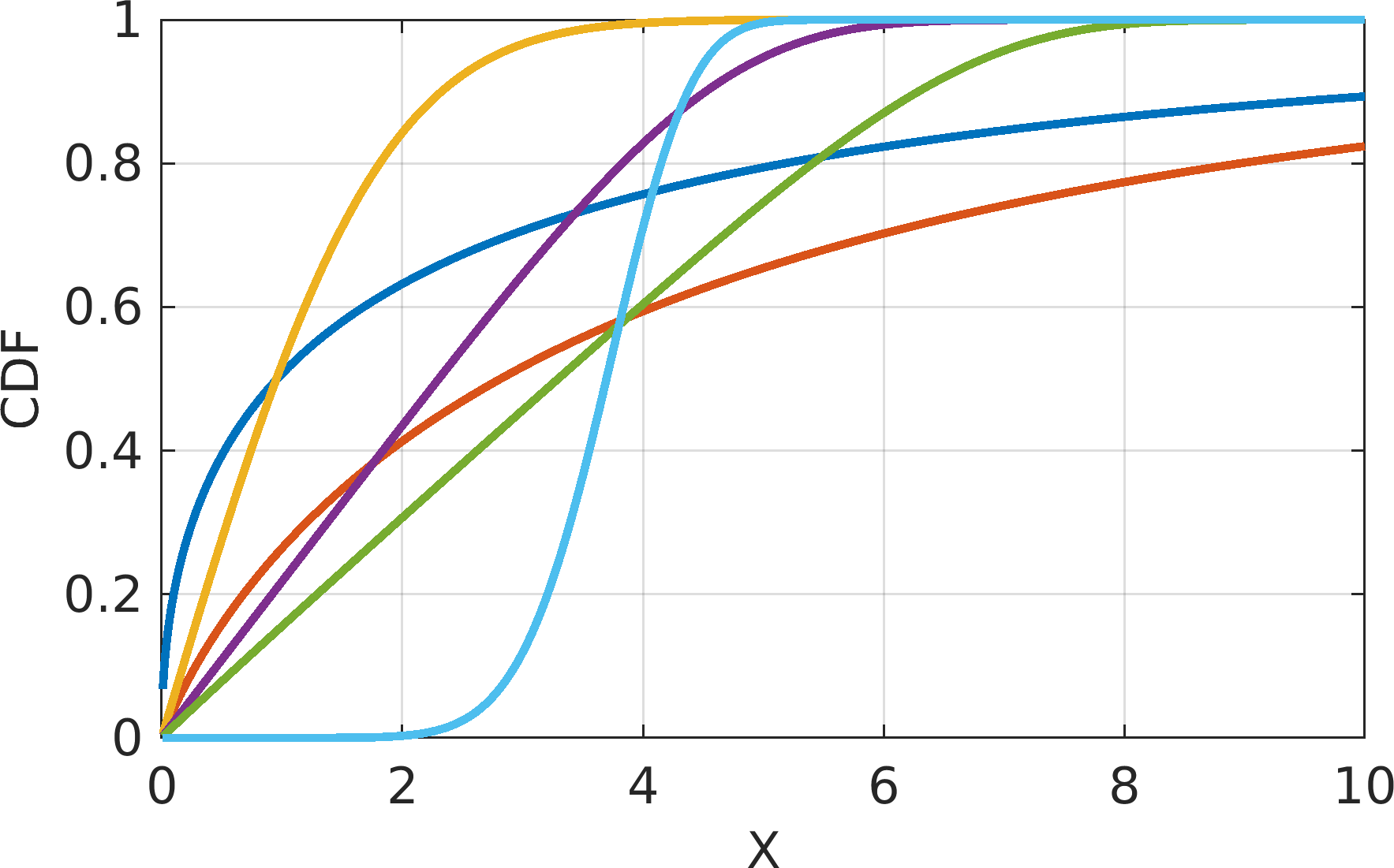
Return the corresponding Cumulative Distribution Function (CDF) of the input random value(s) from the Generalized Gamma distribution.

A variable \(X\) is said to be Generalized Gamma (GenGamma) distributed if its PDF with the scale \(0 < \sigma < +\infty\), shape \(0 < \omega < +\infty\), and shape \(0 < \kappa < +\infty\) parameters is described by the following equation,

\begin{equation} \large \pi(x | \kappa, \omega, \sigma) = \frac{1}{\sigma \omega \Gamma(\kappa)} ~ \bigg( \frac{x}{\sigma} \bigg)^{\frac{\kappa}{\omega} - 1} \exp\Bigg( -\bigg(\frac{x}{\sigma}\bigg)^{\frac{1}{\omega}} \Bigg) ~,~ 0 < x < \infty \end{equation}

where \(\eta = \frac{1}{\sigma \omega \Gamma(\kappa)}\) is the normalization factor of the PDF.
When \(\sigma = 1\), the GenGamma PDF simplifies to the form,

\begin{equation} \large \pi(x) = \frac{1}{\omega \Gamma(\kappa)} ~ x^{\frac{\kappa}{\omega} - 1} \exp\Bigg( -x^{\frac{1}{\omega}} \Bigg) ~,~ 0 < x < \infty \end{equation}

If \((\sigma, \omega) = (1, 1)\), the GenGamma PDF further simplifies to the form,

\begin{equation} \large \pi(x) = \frac{1}{\Gamma(\kappa)} ~ x^{\kappa - 1} \exp(-x) ~,~ 0 < x < \infty \end{equation}

Setting the shape parameter to \(\kappa = 1\) further simplifies the PDF to the Exponential distribution PDF with the scale parameter \(\sigma = 1\),

\begin{equation} \large \pi(x) = \exp(x) ~,~ 0 < x < \infty \end{equation}

1. The parameter \(\sigma\) determines the scale of the GenGamma PDF.
   
2. When \(\omega = 1\), the GenGamma PDF reduces to the PDF of the Gamma distribution.
   
3. When \(\kappa = 1, \omega = 1\), the GenGamma PDF reduces to the PDF of the Exponential distribution.
   

The CDF of the Generalized Gamma distribution over a strictly-positive support \(x \in (0, +\infty)\) with the three (shape, shape, scale) parameters \((\kappa > 0, \omega > 0, \sigma > 0)\) is defined by the regularized Lower Incomplete Gamma function as,

\begin{eqnarray} \large \mathrm{CDF}(x | \kappa, \omega, \sigma) & = & P\bigg(\kappa, \big(\frac{x}{\sigma}\big)^{\frac{1}{\omega}} \bigg) \\ & = & \frac{1}{\Gamma(\kappa)} \int_0^{\big(\frac{x}{\sigma}\big)^{\frac{1}{\omega}}} ~ t^{\kappa - 1}{\mathrm e}^{-t} ~ dt ~, \end{eqnarray}

where \(\Gamma(\kappa)\) represents the Gamma function.

Parameters

[in]	x	: The input scalar or array of the same shape as other array-valued arguments, containing the values at which the CDF must be computed.
[in]	kappa	: The input scalar or array of the same shape as other array-valued arguments, containing the shape parameter ( \(\kappa\)) of the distribution.
[in]	invOmega	: The input scalar or array of the same shape as other array-valued arguments, containing the inverse of the second shape parameter ( \(\omega\)) of the distribution.
[in]	invSigma	: The input scalar or array of the same shape as other array-valued arguments, containing the inverse of the scale parameter ( \(\sigma\)) of the distribution.

Returns

cdf : The output scalar or array of the same shape as other array-valued input arguments of the same type and kind as x containing the PDF of the specified GenGamma distribution.

Possible calling interfaces ⛓

cdf = pm.stats.dist.gengamma.getCDF(x, kappa, invOmega, invSigma)

Example usage ⛓

cd(fileparts(mfilename('fullpath'))); % Change working directory to source code directory.
addpath('../../../../../'); % Add the ParaMonte library root directory to the search path.
 
x = exp(linspace(log(0.01), log(10), 1000))';
 
cdf = zeros(numel(x), 6);
cdf(:,1) = pm.stats.dist.gengamma.getCDF(x, 1.0, 0.5, 0.5);
cdf(:,2) = pm.stats.dist.gengamma.getCDF(x, 2.0, 0.5, 1.0);
cdf(:,3) = pm.stats.dist.gengamma.getCDF(x, 0.5, 2.0, 0.5);
cdf(:,4) = pm.stats.dist.gengamma.getCDF(x, 0.2, 5.0, 0.2);
cdf(:,5) = pm.stats.dist.gengamma.getCDF(x, .14, 7.0, .14);
cdf(:,6) = pm.stats.dist.gengamma.getCDF(x, 2.0, 5.0, 0.3);
 
df = array2table([x, cdf]);
p = pm.vis.PlotLine(df, "colx", 1, "coly", 2:length(df{1,:}), "plot", {"linewidth", 2});
p.subplot.colormap.enabled = false;
p.subplot.ylabel.txt = "CDF";
p.subplot.xlabel.txt = "X";
p.make();
p.savefig("gengamma.getCDF.line.png", "-m4");

Example output ⛓

Visualization of the example output ⛓

Final Remarks ⛓

---

If you believe this algorithm or its documentation can be improved, we appreciate your contribution and help to edit this page's documentation and source file on GitHub.
For details on the naming abbreviations, see this page.
For details on the naming conventions, see this page.
This software is distributed under the MIT license with additional terms outlined below.

1. If you use any parts or concepts from this library to any extent, please acknowledge the usage by citing the relevant publications of the ParaMonte library.
   
2. If you regenerate any parts/ideas from this library in a programming environment other than those currently supported by this ParaMonte library (i.e., other than C, C++, Fortran, MATLAB, Python, R), please also ask the end users to cite this original ParaMonte library.
   

This software is available to the public under a highly permissive license.
Help us justify its continued development and maintenance by acknowledging its benefit to society, distributing it, and contributing to it.

Copyright

Computational Data Science Lab

Author:

Fatemeh Bagheri, May 20 2024, 1:25 PM, NASA Goddard Space Flight Center (GSFC), Washington, D.C.
Amir Shahmoradi, July 19, 2024, 1:07 AM, NASA Goddard Space Flight Center (GSFC), Washington, D.C.