This lecture discusses some of the most important topics in MATLAB plotting, as well as random numbers and Monte Carlo methods in MATLAB.
Lecture Videos
This video is created solely as a reference for the attendants of ICP2017F course at UT Austin. If you did not attend this class, then you may not find this video useful.
Curve plotting in MATLAB
One of the most useful methods of outputting the results of your research and MATLAB projects is plotting. MATLAB is truly the unique best language for plotting data, and in my personal view, no other language comes even close to it (except perhaps, the R programming language which is specifically designed for data analysis and plotting). Here in this lecture, we will only review some of the most important and most useful plotting capabilities in MATLAB.
Plotting simple 2D data
One of the most widely used MATLAB plotting functions is plot(). With this function, plotting x-y data is as simple as it can be. All you need to have is a dataset consisting of X and Y vectors,
>> X = 0:0.1:10;
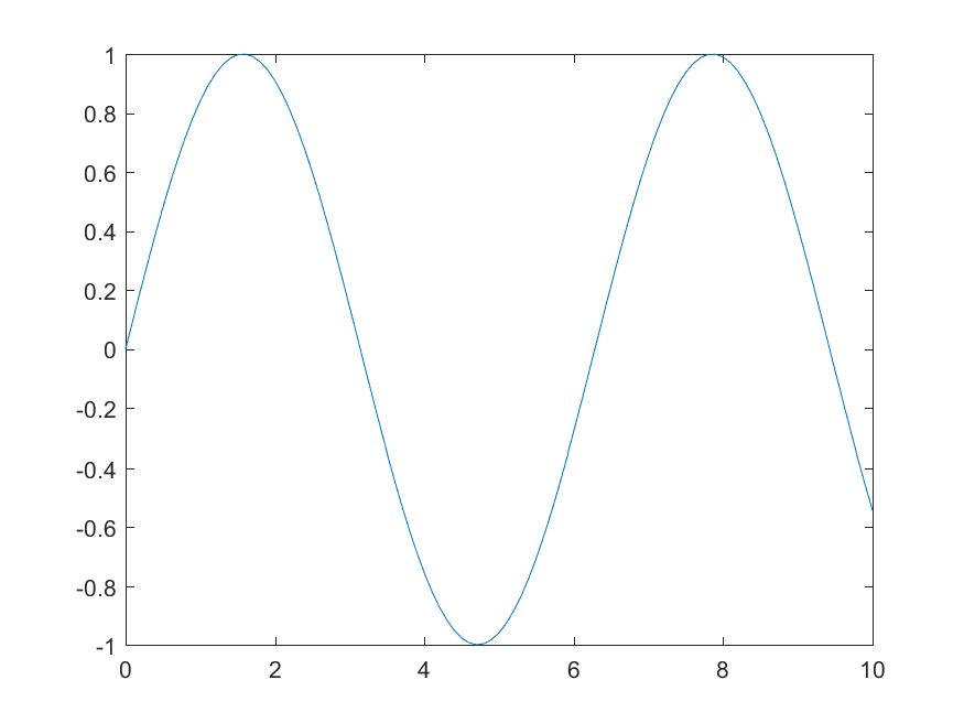
>> plot(X,sin(X));
This will open the following MATLAB figure page for you in the MATLAB environment,
You could also save this figure in almost any format you wish using save() function,
>> saveas(gcf,'sin.png')
Here, gcf refers tothe current figure handle in MATLAB environment. If you wish to add new data to this plot, you could use hold on; command,
>> hold on;
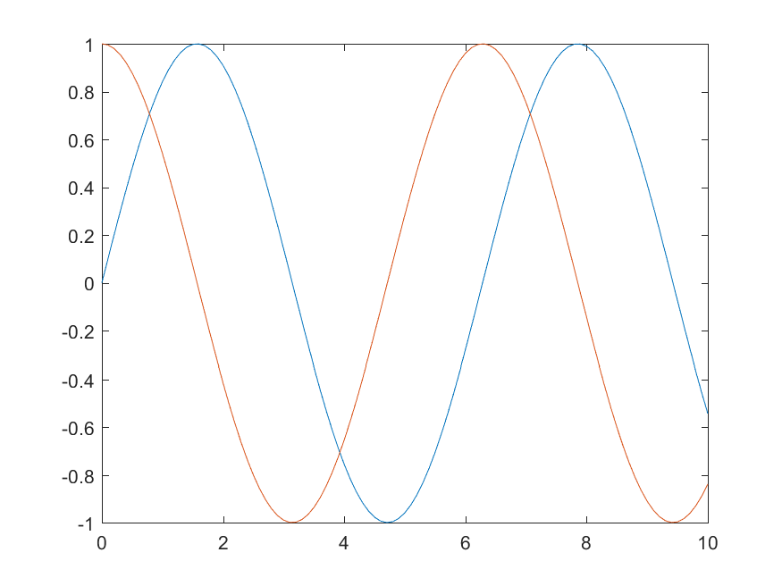
>> plot(X,cos(X));
>> saveas(gcf,'sinCos.png')
This will save the following figure for you, on your local device,
Annotating and decorating your MATLAB plots
Things you can do with MATLAB plotting functions is virtually endless, and there is no way we could cover all of them here in this course. Nevertheless, here are a few useful commands that help you decorate your plots. For example you could add a plot title as well as X-axis and Y-axis labels to your plots by,
>> title('A simple plot of Sin(x) and Cos(X)', 'fontsize', 12)
>> xlabel('X value', 'fontsize', 13);
>> ylabel('Y value', 'fontsize', 13);
Also we could add legends to the plot, explaining what each line represents,
>> legend( { 'Sin(X)' , 'Cos(X)' } , 'fontsize' , 13 , 'location' , 'southwest' );
Note that the fontsize keyword is not necessary. You could simply omit it and MATLAB’s default font size will be used instead.
You could also change the line-width of the borders of the plot, for example, by,
>> set( gca , 'linewidth' , 3 );
Here, gca is a MATLAB keyword that refers to the current active plot in the current active figure. If you wanted to thicken the curve lines themselves, you could simple add the 'linewidth' keyword when calling plot(), along with the desired line width value. You could also determine the line color using color keyword followed by the desired color,
>> hold off; % this closes access to the old figure
>> figure() % this creates a new figure handle
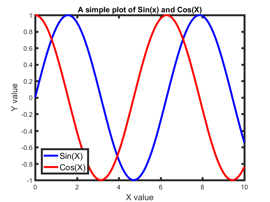
>> plot(X,sin(X),'linewidth',3, 'color', 'blue');
>> hold on;
>> plot(X,cos(X),'linewidth',3, 'color', 'red');
>> legend( { 'Sin(X)' , 'Cos(X)' } , 'fontsize' , 13 , 'location' , 'southwest' );
>> title('A simple plot of Sin(x) and Cos(X)', 'fontsize', 12)
>> xlabel('X value', 'fontsize', 13);
>> ylabel('Y value', 'fontsize', 13);
>> set( gca , 'linewidth' , 3 );
>> saveas(gcf,'sinCosDecorated.png')
This will generate the following figure and save it to your local hard drive,
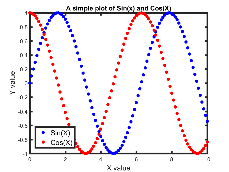
You can also plot the data using different line/ point styles. For example, to plot the same data using points instead of lines, all you need to do, is to add the '.' string to your plot() functions, indicating that you want a scatter plot, instead of line plot,
>> figure() % this creates a new figure handle
>> plot(X,sin(X), '.', 'color', 'blue', 'markersize', 20);
>> hold on;
>> plot(X,cos(X), '.', 'color', 'red', 'markersize', 20);
>> legend( { 'Sin(X)' , 'Cos(X)' } , 'fontsize' , 13 , 'location' , 'southwest' );
>> title('A simple plot of Sin(x) and Cos(X)', 'fontsize', 12)
>> xlabel('X value', 'fontsize', 13);
>> ylabel('Y value', 'fontsize', 13);
>> set( gca , 'linewidth' , 3 );
>> saveas(gcf,'sinCosDecoratedScatter.png')
which will produce and save the following plot,
To learn more about fantastic things you can do with MALTAB plotting functions, see this page.
Other more complex plotting functions in MATLAB
MATLAB, as said above, has a tremendous set of plotting functions, which make it an ideally suited programming language for scientific research. We will learn how to use some of these functions in homework 5. Here on this page, you can find a long list of MATLAB plotting functions and types of plots that you can draw using MATLAB.
Closing figures and plots in MATLAB
for closing the current active figure in MATLAB, you could simply use close(gcf). Here, gcf refers to the current active figure handle. To close all open figures, simply type close all;.
Random numbers in MATLAB
One of the most important topics in today’s science and computer simulation is random number generation and Monte Carlo simulation methods. In the simplest scenario for your research, you may need to generate a sequence of uniformly distributed random numbers in MATLAB. MATLAB has a large set of built-in functions to handle such random number generation problems. All of these functions are collectively named the statistics and machine learning toolbox in MATLAB.
MATLAB has a long list of random number generators. For example, you can use rand() to create a random number in the interval (0,1),
– X = rand returns a single uniformly distributed random number in the interval (0,1).
– X = rand(n) returns an n-by-n matrix of random numbers.
– X = rand(n,m) returns an n-by-m matrix of random numbers.
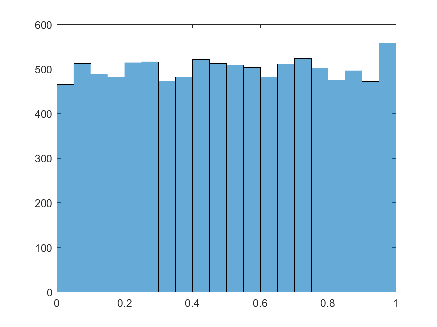
For example, suppose you generated 10000 uniform random numbers,
>> RandomValues = rand(10000,1);
You could test whether the generated random numbers are truly uniformly distributed or not by plotting their histogram,
>> histogram(RandomValues)
which will plot the following figure,
To generate random integer numbers in a given range, you can use randi() function,
– X = randi(imax) returns a pseudorandom scalar integer between 1 and imax.
– X = randi(imax,n) returns an n-by-n matrix of pseudorandom integers drawn from the discrete uniform distribution on the interval [1,imax].
– X = randi(imax,n,m) returns an n-by-m matrix of pseudorandom integers drawn from the discrete uniform distribution on the interval [1,imax].
– X = randi([imin,imax],n,m) an n-by-m matrix of pseudorandom integers drawn from the discrete uniform distribution on the interval [imin,imax].
For example,
>> randi([10 23], 3,2)
ans =
    20    16
    13    17
    18    11
Note that so far, we have only generated uniformly distributed float/integer random numbers. We could however, generate random numbers according to any distribution we wish, that is also supported by MATLAB. For example, a very popular distribution choice, is random number from the Normal (Gaussian) distribution. To get normally distributed random numbers, you can use MATLAB function randn(),
– X = randn returns a random scalar drawn from the standard normal distribution (mean=0,sigma=1).
– X = randn(n) returns an n-by-n matrix of standard-normally distributed random numbers.
– X = randn(n,m) returns an n-by-m matrix of standard-normally distributed random numbers.
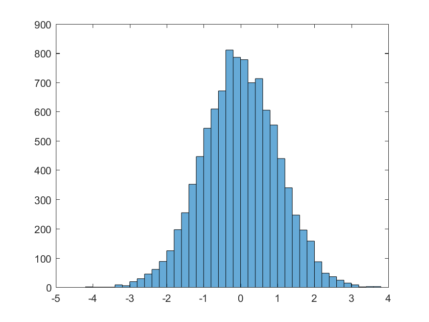
Note that this function generated only standard-normally distributed random values. Therefore, a histogram of 10000 of such values produced by randn() would look something like the following,
>> SNormalValues = randn(10000,1);
>> histogram(SNormalValues);
To get normally distributed random numbers with mean and standard deviation other than the standard normal distribution (μ=0,σ=1), you will have to use another MATLAB builtin function normrnd(),
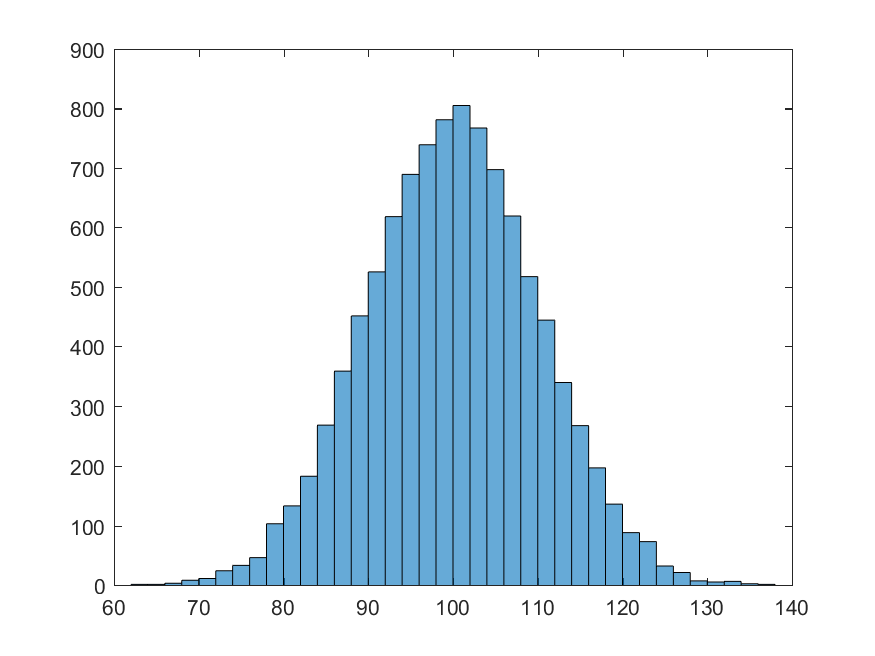
– R = normrnd(mu,sigma) generates random numbers from the normal distribution with mean parameter mu and standard deviation parameter sigma. mu and sigma can be vectors, matrices, or multidimensional arrays that have the same size, which is also the size of R. A scalar input for mu or sigma is expanded to a constant array with the same dimensions as the other input.
– R = normrnd(mu,sigma,m,n,…) or R = normrnd(mu,sigma,[m,n,…]) generates an m-by-n-by-… array. The mu, sigma parameters can each be scalars or arrays of the same size as R.
NormalValues = normrnd(100, 10, 10000, 1);
>> histogram(NormalValues)
The deterministic aspect of randomness in MATLAB
There is a truth about random numbers and random number generators and algorithms, not only in MATLAB, but in all programming languages, and that is, true random numbers do not exist in the world of programming!
What we call a sequence of random numbers, is simply a sequence of numbers that we, the user, to the best of our knowledge, don’t know how it was generated, and therefore, the sequence looks random to us, but not the to the developer of the algorithm!. To prove this, type the following code in a MATLAB session,
>> rng(135);
>> rand()
ans =
    0.8844
>> rand()
ans =
    0.0771
>> rand()
ans =
    0.5492
>> rand()
ans =
    0.8296
Here, the function rng() controls the random number generation algorithm using the input positive integer number. The truth is that every algorithm for random number generation is deterministic and starts from an input integer number, called the seed of random number generator, to construct the sequence of random numbers. This means, that if we set the random number seed to a fixed value before we call the random number generator every time, then we will always get the same fixed random value (in fact, it is not random anymore!),
>> rng(135);
rand()
ans =
    0.6613
>> rng(135);
rand()
ans =
    0.6613
>> rng(135);
rand()
ans =
    0.6613
>> rng(135);
rand()
ans =
    0.6613
Note that, every time you restart MATLAB, the random number generator seed is set back to the default value, nor matter what you set it to in the last time. This means that every time you open MATLAB, type rand(), you will get the exact same random number as in the last time you opened MATLAB. To avoid this problem, you can use,
>> rng('shuffle')
which seeds the random number generator based on the current time in the CPU. Thus, rand, randi, and randn will produce a different sequence of numbers after each time you call rng(‘shuffle’).
Sometimes however, this is not the desired behavior. For example, you want the results of your code to be reproducible. In those cases, it is actually good to initialize the seed of the random number generator in MATLAB to some pre-specified number, so that every time you run your code, you get the exact same result as before. To learn more about the seed of random number generators in MATLAB, visit this page.
Creating random permutation of numbers
There is a useful MATLAB function called randperm() that generates a random permutation of numbers for the user,
– p = randperm(n) returns a row vector containing a random permutation of the integers from 1 to n inclusive.
For example, if we wanted to get a sequence of random numbers within the range from 1 to a given maximum integer n, say n=10, in an arbitrary order, we could use this function,
>> randperm(10)
ans =
     8     5     2     1    10     6     4     3     9     7
>> randperm(10)
ans =
     4     8     1     3    10     2     5     7     9     6
>> randperm(10)
ans =
     6     1     2     4     5     8     7     3    10     9
Note that every time you call the function, you would get a new random permutation of the requested sequence of numbers.

